Validating the Skills of Satellite Rainfall Products and Spatiotemporal Rainfall Variability Analysis over Omo River Basin in Ethiopia

Elsabet Temesgen Asefw; Getachew Tesfaye Ayehu

doi:doi:10.11648/j.hyd.20241202.13

Research Article |

| Peer-Reviewed

Validating the Skills of Satellite Rainfall Products and Spatiotemporal Rainfall Variability Analysis over Omo River Basin in Ethiopia

Elsabet Temesgen Asefw^*

, Getachew Tesfaye Ayehu

Published in Hydrology (Volume 12, Issue 2)

Received: 26 March 2024 Accepted: 17 June 2024 Published: 29 June 2024

Views: Downloads:

Download PDF

Share This Article

Twitter
Linked In
Facebook

Abstract

Recently created long-term and regionally dispersed satellite-based rainfall estimates have emerged as crucial sources of rainfall data to assess rainfall's spatial and temporal variability, particularly for data-scarce locations. Objective (the general): The purpose of this paper is to assess the skills of nine selected satellite rainfall estimates i.e., (ARC 2.0, TRMM 3B42, CHIRPS v. 2.0, TAMSAT 3.1, CMORPH v. 1.0 adj., PERSIANN CDR and DNRT, and MSWEP v. 2.2) and understand Spatio-temporal variability of rainfall over the Omo River basin using the best performing product. Method: The validation analysis was done by using a point-to-grid-based comparison test at different temporal accumulations. MSWEP was selected as the best product to analyze the long-term trend and variability of rainfall over the Omo-River basin from 1990-2017. The coefficients of variation (CV) and the standardization rainfall anomalies index (SRAI) were used to examine rainfall variability, while the Mann-Kendall (MK) and Sen slope estimators were used to examine the trend and magnitude of rainfall patterns. Results: The overall statistical, categorical, and volumetric validation index results show that the MSWEP is the best performing rainfall product followed by CHRIPS, 3B42, and TAMSAT according to their order of appearance than the remaining products (i.e., ARC, RFE, PER CDR, PER DNRT, and CMORPH). The CV result with the relatively highest monthly variability (CV > 30%) was observed in some southern, northern, southeastern, and central parts of the study area. In general, the overall annual CV shows almost no variation in the entire basin except in the lower part because of the region's prevalent topographic variances, which ranged from 3455 to 352 m.a.s.l. In addition, the highest seasonal positive and negative anomalies are observed in each season in the entire basin. These abnormalities can result in significant floods and droughts that unquestionably influence the basin and its resources. Conclusion: In general, the basin has an increasing trend in the southern portions and a declining trend in the central to northern tip parts of the basin, as can be observed from the annual average MK trend tests. The basin has experienced a greeter variation but is not significant except in some parts of the basin.

Published in	Hydrology (Volume 12, Issue 2)
DOI	10.11648/j.hyd.20241202.13
Page(s)	36-51
Creative Commons	This is an Open Access article, distributed under the terms of the Creative Commons Attribution 4.0 International License (http://creativecommons.org/licenses/by/4.0/), which permits unrestricted use, distribution and reproduction in any medium or format, provided the original work is properly cited.
Copyright	Copyright © The Author(s), 2024. Published by Science Publishing Group

Keywords

Rainfall, MSWEP, Trends, CHIRPS

1. Introduction

In recent decades the availability of surface and groundwater, as well as global and regional water cycles, are all impacted by climate change and fluctuation

[1]

. The negative effects of spatiotemporal variability of rainfall, which have a significant impact on water resources, have become a bottleneck for agricultural and livestock production

[2]

. According to

[3]

, this condition has particularly most pronounced in Eastern African countries, due to its complex terrain, latitudinal location, and the influence of regional and global atmospheric circulation. Ethiopia has a wide range of climates, rugged geography, and a lot of water resources

[4]

. Spatiotemporal dynamics of the water resources are characterized by multi-weather systems rainfall of the country.

Rainfall is the key driving force in hydrological studies, required to understand the complexity of the water cycle and to manage water resources

[5]

. The direction, intensity, and trends of rainfall across locations and seasons fluctuate throughout time, from days to day

[6, 7]

. Due to its significant influence on both socioeconomic and environmental problems, the variability and trend analysis of rainfall need necessary attention to be studied. These issues are more prevalent in inaccessible regions like Ethiopia's highlands and lowlands, where rainfall is extremely variable over short distances. Therefore, having access to reliable and accurate ground-based observed rainfall data in a particular planning unit or region provides significant advantages. However, in many parts of the world, particularly in the least developed countries, accurate and consistent observed rainfall data are limited mainly due to poor and uneven, and sparse distribution of rain gauge stations network across a given geographical area

[8, 9]

. Nowadays, technological advancements in remote sensing such as satellite-based rainfall estimates have become good alternatives and better options to bridge the gap and un input data sources for many hydro meteorological analyses, especially for data-sparse regions

[9, 10]

. For this reason, there is a need to assess the skills of nine selected satellite rainfall estimates i.e., (ARC 2.0, TRMM 3B42, CHIRPS v. 2.0, TAMSAT 3.1, CMORPH v. 1.0 adj., PERSIANN CDR and DNRT, and MSWEP v. 2.2) and understand Spatio- temporal variability of rainfall over the Omo River basin using the best performing product.

2. Description of the Study Area

The Omo River (additionally known as Omo-Gibe or Bottego river basin) is placed in Southwestern Ethiopia and its miles are the biggest river outdoors the Nile Basin. It lies in the 4°30′ to 9°00′ N range and 35° 00′ to 38°E longitude with a mean altitude of 2800 m a.m.s.l. The climate of the Omo River Basin varies from a hot arid climate in the south to a tropical humid in the highlands that include the extreme north and northwestern part of the basin

[11]

. Moreover, the seasonal rainfall distribution within the Omo Gibe River Basin arises out of the annual migration of the ITCZ.

2.1. Data Collection and Analysis

Download: Download full-size image

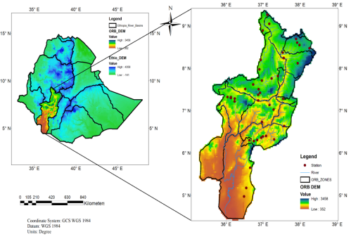
Figure 1. Geographical location of the study area data source from (SRTM DEM data is being housed on the USGS Earth Explore).

To comprehend the overall aspects of the problem under investigation, the study utilized primary data sources. These data sources are meteorological records of climate data (rainfall data) from the Ethiopian Meteorology Institute (EMI) and satellite rainfall estimation products (SREPs) which are freely available on the climate data analysis tool (CDT) and the web for the specified study site. Rainfall data was selected from 2000-2020 for 42 ground stations and the presence of observed data was checked using CDT (climate data analysis tool) and the result shows that most of the station data available from 75% to 100%. This value indicates good historical data available for the selected observed ground stations.

2.2. Satellite Rainfall Data

SRE products are increasingly available with almost global coverage and the supply of those products is becoming cost-effective sources for many applications

[12]

. Most of SREPs are combined products of reanalysis, rain gauge data, and remote sensing estimation, for this desired specific objective nine satellite rainfall estimation products are selected depending on their high spatial resolution, relatively long time series, and freely available. A summary of the satellite rainfall products is given below in Table 1.

3. Methodology

3.1. Validation SREP with Gauge Rainfall Data

The spatial patterns of nine satellite products were evaluated and compared with 42 rain gauge data from 2000-2020. All of the SRE products taken into consideration were statistically evaluated to determine how well they could detect rainfall on a daily, decadal, monthly, seasonal, and annual basis. The comparison between gridded satellite rainfall estimates and ground rainfall observations can be made using either grid- to-grid or point-to-grid comparison methods.

Table 1. Satellite rainfall estimation products used in this study and their spatial and temporal Characteristics.

The first method requires interpolation of the gauge data with the grid data, where the grid gauge data is compared with the grid data of global precipitation estimates; however, converting points to meshed interpolated data causes errors due to uneven geospatial distribution interpolation

[12-14]

Thus, this study has used point-to-grid comparison approaches.

3.1.1. Statistical Evaluation Method

Correlation coefficient (r): - Indicate the relationship between observed rainfall data and the SREPs products. Where Gr is ground observed rainfall data and Sr is satellite rainfall estimation. The range of values of r is from +1 to −1, in which the value of 0 indicates that there is no linear relationship between the satellite-derived rainfall estimation and in-situ observations, the value 1 indicates perfect positive linear correlation and the value −1 implies a perfect negative linear correlation.

r = \frac{\sum (Gr - Grmean) (Sr - Srmean)}{\sqrt{\sum {(Gr - Grmean)}^{2} \sqrt{\sum {(Gr - Grmean)}^{2}}}}

(1)

Coefficient of determination (R²): - describes the proportion of the variance in observation data by the satellite estimation. It is the magnitude linear relationship between the observed and the satellite values. R ² ranges from 0 which indicates poor model performance to 1 which indicates best model performance and typical values greater than 0.6 are considered acceptable model performance.

R^{2} = {(\frac{\sum (Gr - Grmean) (Sr - Srmean)}{\sqrt{\sum {(Gr - Grmean)}^{2} \sqrt{\sum {(Gr - Grmean)}^{2}}}})}^{2}

(2)

Mean Error (ME) and Mean Absolute Error (MAE): - Mean bias error (ME) (ranges from − ∞ to ∞) and mean absolute error (MAE) (ranges from 0 to ∞) measures the average magnitude of estimation error and the perfect score for these statistics is zero. Positive and negative ME value indicates an overestimation and underestimation of SRE data products, respectively

[15]

ME=1/n∑ (Sr−Gr)(3)

MAE = \frac{1}{n} \sum_{i = 1}^{n} Gri - Sri

(4)

Root Mean Square Error (RMSE): - is a measure of the differences between satellite observation and the actual values measured by rain gauge (measure the average error magnitude) or it is one of the error indices and use to measure of the difference between observed and SREPs values. The value of 0 represents the perfect fit.

RMSE = \sqrt{\sum_{i = 1}^{n} \frac{{(Gr - Sr)}^{2}}{n}}

(5)

Bias is a measure of how the average satellite rainfall magnitude compares to the ground rainfall observation.

A value of 1 is the perfect score. A bias value above (below) 1 indicates an aggregate satellite overestimation (underestimation) of the ground precipitation amounts.

Bias= ∑Sr/ ∑G……(6)

Nash–Sutcliffe efficiency coefficient: - It determines the relative magnitude of variance of residues and measured data. NSE values range between −∞ and 1, with value 1 indicating a perfect fit between the satellite-based and observed rainfall.

NSE = \frac{{(\sum_{i = 1}^{n} (Sri - Gri))}^{2}}{{(\sum_{i = 1}^{n} (Gri - Sri))}^{2}}

(7)

Percent Bias (PBIAS): It is calculated between the observed and SREPs and it indicates the systematic error (larger or smaller than observed) in rainfall amount (Measure the average tendency of the SREPs). Range value between (Positive values of PBIAS indicate an overestimation of the rainfall quantity, whereas negative values show an underestimation of the rainfall quantity.

PBIAS = \frac{\sum_{i = 1}^{n} (Sri - Gri) * 1}{\sum_{i = 1}^{n} Sr * 100}

(8)

3.1.2. Categorical Performance Indices

To evaluate the performance of satellite rainfall products, four categorical statistical indices were used, the probability of detection (POD), false alarm ratio (FAR), Heidke skill score (HSS) and Critical successes index (CSI)

[16]

. POD measures the rain events that were correctly detected by the satellite; FAR measures the rain events that were incorrectly detected; HSS were used to assess the accuracy of SREPs in identifying rainfall days (i.e., days with ≥ 1mm) and CSI describing the overall skill of the satellite products relative to gauge observation. The ideal values of POD, FAR, and CSI range from 0 to 1, with 1 being a perfect measure for POD and CSI while 0 for FAR and (-∞-1) for HSS.

POD = \frac{H}{H + M}

(9)

FAR = \frac{F}{F + M}

(10)

CSI = \frac{H}{H + M + F}

(11)

HSS = \frac{2 (H * CD - F * M)}{(H + M) (M + CD) + (H + F) (F + CD)} \dots .

(12)

Every grid cell is classified as a hit (H) when a rainfall recorded by both satellite and rain gauge; miss (M) when rain observed by only the rain gauge; and false alarm (F) when rain is documented only by satellite. To define whether there is rain or no rain pixels, a threshold value 1.0 mm/day was adopted

[16]

. The categorical statistical indices are given below: - where CD stands for corrected negative that could occur by chance. Note that when a threshold is set, a wet day occurs when an amount greater than the set threshold was recorded. The ability of SREs to detect rainy days, defined here as days with a rainfall total of more than 1 mm, was assessed based on the contingency Table 2 using dichotomous metric.

Table 2. The 2 × 2 contingency table for comparing the rainy days in gauge and satellite estimate. A day is considered rainy if 1 mm of rainfall or more is recorded.

	Gauge ≥ 1 mm	Gauge < 1 mm
Satellite ≥ 1 mm	Hit (H)	False alarm (F)
Satellite < 1 mm	Miss (M)	CD

3.1.3. Volumetric Validation Indices

Is an extension of the categorical table, it includes (i) the volumetric hit index (VHI), (ii) the volumetric false alarm ratio (VFAR), and (ii) the volumetric critical success index (VCSI) that were proposed by

[17]

have been adopted to evaluate the volumetric performance of the selected satellite rainfall products.

VHI = \frac{\sum_{i = 1}^{n} (Sri (Sri > t Gri > t))}{\sum_{i = 1}^{n} (Sri \ (Sri > t Gri > t)) + \sum_{i = 1}^{n} (Gri \leq t Gri > t)}

(13)

Where VHI is the volume of correctly detected rainfall by the satellites relative to the volume of the correctly detected satellites and missed gauge observations.

VFAR = \frac{\sum_{i = 1}^{n} (Sri \ (Sri > t Gri > t))}{\sum_{i = 1}^{n} (Sri \ (Sri > t Gri > t)) + \sum_{i = 1}^{n} (\frac{Sri}{Sri > t Gri \leq t})}

(14)

Where VFAR is the volume of false rainfall by the satellites relative to the sum of rainfall by the satellite

VCI \frac{\sum_{i = 1}^{n} (Sri \ (Sri > t Gri > t))}{\sum_{i = 1}^{n} (Sri \ (Sri > t Gri > t)) + \sum_{i = 1}^{n} (Sri \ (Sri \leq t Gri > t)) + \sum_{i = 1}^{n} (Sri \ (Sri > t Gri \leq t))}

(15)

Where VCSI is the overall measure of volumetric performance. Here S is satellite rainfall estimates, G is gauge observations, i =1 to n and n is the sample size, and t is the threshold values (t = 1 mm in this study).

3.1.4. Quantile Validation Indices

It is used to detect the volumetric skills of the precipitation products for different extreme precipitation thresholds i.e., 50%, 80%, and 90% quantiles of reference data

[17]

. But for this study chosen from the above quantiles select 80% precipitation thresholds for volumetric evaluation metrics.

Quantile probability of detection (QPOD): _is defined as the probability of detection (POD; see

[18, 17]

above a certain threshold.

QPOD = \frac{\sum_{i = 1}^{n} I (\frac{Sr}{Sr} > t Gr \geq t)}{\sum_{i = 1}^{n} I (\frac{Sr}{Sr} > t Gr > t) + \sum_{i = 1}^{n} I (\frac{Gr}{Sr} \geq t Gr > t)}

(16)

Were, I the indicator function. The QPOD represents the ratio of the number of correct identifications of precipitation above a given threshold to the total number of precipitation occurrences above the same threshold as indicated by the reference. And The QPOD ranges from 0 to 1, with 1 being the perfect QPOD. For all products, the probability of detection reduces as the threshold increases.

Quantile False Alarm Ratio: _Quintile false extreme alarm ratio (QFAR) is defined as the false alarm ratio above a certain threshold:

QFAR = \frac{\sum_{i = 1}^{n} I (\frac{Sr}{Sr} > t Gr \leq t)}{\sum_{i = 1}^{n} I (\frac{Sr}{Sr} > tGr > t) + \sum_{i = 1}^{n} I (\frac{Sr}{Sr} > tGr \leq t)}

(17)

The QFAR represents the ratio of the number of false identifications of precipitation above a given threshold to the total number of correct and false occurrences over the same threshold as indicated by the reference. The QFAR ranges from 0 to 1, with 0 being the perfect QFAR.

Quantile critical success index (QCSI) given as

QCSI = \frac{\sum_{i = 1}^{n} I (\frac{Sr}{Sr} > t Gr > t)}{\sum_{i = 1}^{n} I (\frac{Sr}{Sr} > t Gr > t) + \sum_{i = 1}^{n} I (\frac{Gr}{Sr} \leq t Gr > t) + \sum_{i = 1}^{n} I (\frac{Sr}{Sr} > t Gr \leq t)}

(18)

3.2. Spatio Temporal Rainfall Variability

For this case investigate the spatiotemporal variability and trends of rainfall across ORB, the coefficient of variation (CV) method, the standardized rainfall anomaly (SRA), and trend analysis are the following computations were used to analyze the spatial and temporal variability of annual, seasonal, and monthly rainfall for the study site. The study area's spatial variability of rainfall was developed using the standard kriging interpolation approach in ArcGIS 10.8, seasonal, yearly, and monthly areal rainfall variations were created after the locations of the rain gauge stations for the basin were plotted. When compared to deterministic interpolation techniques like the inverse distance weighted and spline methods, the conventional kriging approach is believed to perform better

[19]

3.2.1. Coefficient of Variation

Generated the coefficient of variation (CV), which was then utilized to study the spatiotemporal variability of annual, seasonal, and monthly rainfall for each pixel given by

CV = \frac{σ}{μ} * 100

(19)

Where CV is the coefficient of variation; 𝜎 is the standard deviation and 𝜇 is the mean precipitation. The CV measures an area's overall rainfall record variability this variability is divided into three categories: low (CV < 20), moderate (20 CV 30), and high (CV >30)

[20-22]

3.2.2. Standardized Rainfall Anomaly Index

Standardized anomaly index (SARI) is used as a descriptor of rainfall variability and it indicates the number of standard deviations that a rainfall event deviates from the average of the considered years

[23]

. It was also used to determine the frequency of dry and wet years in the record and used to assess the frequency and severity of droughts

[10]

. It indicates the departure from the long-term mean with negative values representing periods of below-normal rains (droughts) while positive values reflect above-normal rains (food risk).

Za = \frac{Xi - Xi mean}{σ}

(20)

Where Za is the standard rainfall anomaly; Xi is an annual rainfall of a particular year; Xi is the mean annual rainfall, and 𝜎 is the standard deviation over a period of observations (20 years in our case). A pixel with a negative value of Za represents periods of below-normal rains (drought) while a positive value indicates above-normal rains (with the possible risk of food).

SAI value is classified as extremely wet (SRAI >2), very wet (1.5≤ SRAI ≤1.99), moderately wet (1≤ SRAI≤1.49), near normal (−0.99 ≤ SRAI ≤ 0.99), moderately dry (−1.49 ≤ SRAI ≤ −1), severely dry (−1.99 ≤ SRAI ≤ −1.5) and extremely dry (SRAI ≤ −2)

[23, 24]

(i). MK Trend Analysis

One of the often-employed techniques for identifying a climate trend in time series data is the MK trend test. The MK test's specifics are detailed in

[25]

. The MK test is designed to identify trends in annual and seasonal bases of climate parameters that are monotonically (growing or decreasing). Sen's estimator and the Mann-Kendall (MK) trend test were used to examine whether there had been a long-term change in both the rainfall and temperature indices. The MK test's ability to detect annual and seasonal trend changes is less impacted by climate outliers

[7]

. However, if there is an auto correlation in the time series data, the MK test result could contain some mistake. To solve this issue, a pre-whitening method was carried out with no modifications, and there was no detectable serial autocorrelation at all lags. Based on seasonal and annual rainfall data from 1990 to 2017 in the ORB, the MK test from the Z value and trend from Sen's slope estimation was derived after the serial autocorrelation test. The test based on S statistics and each paired observed values Dj (j > k) of the random variable will be inspected to find out whether Dj > Dk or Dj < Dk.

S = \sum_{i = 1}^{n - 1} \sum_{j = i + 1}^{n} sgn (Dj - Di)

(21)

where Dj and Di are the sequential data values and n is the length of the data set and Sgn

Sgn (Dj - Di) = \begin{matrix} 1 if (Dj - Di) > 0 \\ (0 if (Dj - Di) = 0) \\ - 1 if (Dj - Di) < 0 \end{matrix}

(22)

If the dataset is identically and independently distributed, then the mean of S is zero and the variance of S is given by:

Var (S) = \frac{[n (n - 1) (2 n + 5) - \sum_{i = 0}^{m} ti (ti - 1) (2 ti + 5)]}{18}

(23)

Where, n is the length of the dataset, m is the number of tied groups (a tied group is a set of sample data having the same value) in the time series and tⁱ is the number of data points in the it^h tied group. According to Mann-Kendall, the null hypothesis H0 states that a data series is serially independent and identically distributed with no monotonic trend. The alternative hypothesis H1 is that the data follows a monotonic trend. In a two-sided test for trend at a significance level of 𝛼, H0 should be rejected and H1 is accepted if |Z| > z 𝛼 ∕2, where FN (z 𝛼 ∕2) is the standard normal cumulative distribution function, and Z is the test statistic used to identify the direction of the trend and its significance. The Z statistics are calculated using eq 24.

Z = (\begin{matrix} \frac{S + 1}{\sqrt{Var (S)}} for s < 0 \\ 0 for S = 0 \\ \frac{s - 1}{\sqrt{Var (S)}} for S > 0 \end{matrix})

(24)

The Z is the standard statistics test. The statistical significance level of the trend variation was evaluated using the Z value. A positive MK statistic (Z > 1.96) depicts a significant increasing trend, whereas a negative (Z < -1.96) indicates a significantly decreasing trend, at the α = 0.05 level of significance

[26]

(ii). Sen's Slope Estimator

Sen's slope estimator was also used to calculate the rate of change of the trend to evaluate the relative strength of the MK trend test in time series data

[26]

. Sen's slope estimations are frequently employed to estimate the size of trends in hydro-climate time series. In contrast to linear regression, it reduces the impact of missing values or outliers on the slope. Equation 20 uses the nonparametric Sen's estimator of the slope to calculate the magnitude of the monotonic trend in the hydrologic time series.

Q = median (\frac{Di - Di}{j - i})

(25)

Where, β represents the median value of the slope values between data measurements Di and Dj at the time steps i and j (i, j) respectively. The positive value of β indicates an increasing trend whereas the negative value of β indicates a decreasing trend. The sign of β reflects the data trend direction, whereas its value indicates the steepness of the trend (Adisu et al., n.d.).

For all I < j……… (j = 2..., n and i = 1, n−1

Yt = Dt -

βt(26)

Where Yt is the detrended series, Dt is the original data series value at time t and β is the slope.

4. Results and Discussion

4.1. Daily Validation

Satellite rainfall estimation data were compared to all gauge rainfall data daily. All SREPs performed poorly according to the majority of statistical indicator indices. The value of Pearson’s correlation coefficient at the daily time scale (CC) showed a poor relationship with all satellite rainfall estimation products. This condition was also proved by

[11, 27]

, on all satellite rainfall estimation products.

As can be seen in Table 2 a good relationship was performed by TAMSAT at the value of CC (0.339) with a bitter coefficient of determination (R² = 0.115).

Table 3. A statistical summary of the daily comparison of SREPs with all observed ground rainfall data.

Name	ARC	CHRIPS	CMORPH	MSWEP	PE CDR	PER DNRT	RFE	TAMSAT	3B42	Perfect. Score
CORR	0.242	0.246	0.316	0.311	0.286	0.286	0.255	0.339	0.318	1
R2	0.06	0.06	0.10	0.10	0.08	0.08	0.07	0.11	0.10	1
BIAS	0.733	1.084	0.952	0.991	0.916	1.249	0.827	1.115	1.071	1
PBIAS	-26.7	8.391	-4.778	-0.862	-8.367	24.88	-17.283	11.482	7.132	0
ME	-1.0	0.322	-0.183	-0.033	-0.322	0.956	-0.664	0.441	0.279	0
MAE	4.354	5.229	4.429	4.477	4.414	5.205	4.353	4.618	4.76	0
RMSE	9.241	10.365	9.137	8.99	8.398	10.194	9.053	8.674	9.518	0
NSE	-0.32	-0.659	-0.275	-0.254	-0.086	-0.603	-0.264	-0.16	-0.38	1
POD	0.468	0.448	0.69	0.712	0.772	0.84	0.692	0.705	0.7	1
POFD	0.153	0.165	0.25	0.28	0.361	0.415	0.286	0.269	0.279	0
FAR	0.378	0.407	0.404	0.423	0.464	0.478	0.433	0.414	0.418	0
CSI	0.364	0.343	0.47	0.468	0.463	0.475	0.453	0.471	0.466	1
HSS	0.334	0.299	0.425	0.41	0.373	0.372	0.387	0.416	0.403	1

CC (0.318, 0.316, 0.311, 0.286, and 0.286) was obtained with a finer R² (0.10, 0.09, 0.096, 0.08, and 0.081) by 3B42, CMORPH, MSWEP, PERSSION CDR, and DNRT, respectively, with a small bet difference. According to

[28]

), the TAMAST product outperforms PERSSION, RFE, and CHRIPS over ORB at all-time scales, but only at the daily time scale, as seen in our study. The validation assessment between SREPs and gauge rainfall for each day was processed on a basin scale from 2000 to 2020. As shown in the scatter plot in Figure 2, all SREPs scored low in agreement with observed gauge data due to poor quality control, consistency, and scarcity, as well as their geographical location. This basin's geographical range ranges from 352 – 3458 m.a.s.l., as supported by

[11, 28-30]

. TAMSAT, PER CDR, DNRT, 3B42, CHRIPS, CMORPH1.0adj, and MSWEP in CDF, however, there is a strong linear correlation with estimation data across 3B42, MSWEP, CMORPH, and PER DNRT from the remaining SREPs.

Download: Download full-size image

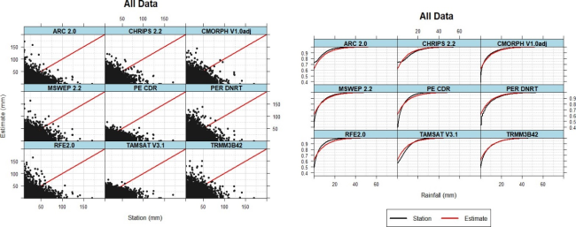
Figure 2. Daily comparison scatter plot and CDF between each SREPs and observed ground rainfall data over Omo River Basin from 2000 to 2020.

4.2. Dekadal Validation

The daily precipitation and SREPs data were combined to create decadal rainfall data, which was then used to evaluate both on a decadal time scale. The overall performance of the SREPs at decadal time scales. CHIRPS 2.0 had a relatively higher correlation value (r = 0.687) with a perfect score POD (1.00), followed by MSWEP, TAMSAT, 3B42, CMORPH, PER CDR, PER DNRT, RFE, and ARC (r = 0.669, r = 0.662, r= 0.641, r = 0.649, r = 0.6, r = 0.605, r = 0.557). All SREPs have a good model performance coefficient of determination (R² = 0.47, 0.447, 0.43, 0.41, and 0.27, respectively). CHRIPS 2.0 has a lower RMSE than the others, with a range of 32.283 – 40.587. ARC 2 and TAMSAT 3.1, as well as CMORPH v1.0 adj, scored relatively medium PODs with the lowest VHI and VCSI values among all SREPS. And all SREPs scored a higher FAR with relative CSI values above 0.795, which analyze the overall skill of the satellite products relative to gauge observation. In contrast, the majority of SRE products were found to have a nearly good bias (bias of 0.733). While sectored at a perfect bias of 0.99 and flowing by PER CDR, CMORP v1.0adj, RFE, and ARC with slightly underestimated observed rainfall, CHRIPS 2.2, TRMM 3B42, TMASAT 3.1, and PER DNRT are overestimated by a small threshold based on the observed data.

4.2.1. Monthly Validation

The monthly correlation of satellite rainfall estimation products was evaluated with gauged rainfall data from 2000–2020, as displayed in Table 4. The result shows CHRIPS had a better relationship with gauged rainfall data than the others and flowed from MSWEP 2.0, TMASAT 3.1, and 3B42. However, CMORPH1.0adj, PERDNRT, PERCDR, RFE, and ARC show a medium level of agreement with the station compared to others. Moreover, comparisons based on a perfect monthly average bias were scored by MSWEP with a slight underestimate from gauged data, which is similar to decadal outputs, and flowed by CHRIPS with a slight overestimate from ground station data. Besides, PER CDR, CMORPH1.0adj, RFE, and ARC show that ground station data is underestimated, while 3B42, TMASAT3.1, and PER DNRT are overestimated. In addition to this, the negative PBIAS scored MSWEP, CMORPH1.0adj, PER CDR, RFE, and ARC, which are underestimated, and the positive PBIAS scored CHRIPS, 3B42, TAMSAT, and PER DNRT, which overestimate rainfall quality.

To verify satellite rainfall estimation products concerning detecting heavy rainfall rates at different temporal accumulations, it should be noted that extremes can be defined based on different viewpoints. In this paper, "heavy extreme rainfall rate" is defined as rainfall rates above the 80% quantile; this condition is proven by

[31]

. As shown in Table 3, the ratio of correct detections above a certain threshold to total occurrences above the same threshold is denoted by the reference "QPOD." Except for ARC, CMORPH1.0adj, and PER CDR, all SREPs have a higher QPOD of 0.861 in this case. All SREPs scored the best QFRA above a certain threshold. Furthermore, those with a lower QCSI received ARC and RFE, while those with a higher QCSI received a perfect QCSI with relative value. To verify more, we need additional information to get a clearer understanding of the capability of satellite rainfall estimation products with gauge rainfall data. In this case, the scatter plot and CDF give a better description map for individual products. As can be seen in Figure 3, all SREPs have good aggregates with ground station data. However, ARC and RFE exhibit underestimation for all accumulation periods over the study area. MSWEP2.0, CHRIPS, 3B42, TAMSAT, and PER CDR demonstrate a good relationship between station and estimation data, with low under- and overestimation. But some satellite rainfall estimation products like PER and DNRT exhibit high threshold overestimates from ground station data.

4.2.2. Seasonal & Annual Validation

SREPS must be validated further using gauge rainfall data from different accumulation time series. Overall, the seasonal Bega, Belg, and Kiremt validation results show that MSWEP performed well in detection and flow, as indicated by 3B42, CMORPH1.0adj, CHRIPS, and TAMSAT, respectively.

As displayed in Figure 4, the annual compression between SREPs with surface station data over the Omo basin the results show that MSWEP outperforms all other SREPs in all metric indices. It has a better CC, a perfect bias, a negative percent of bias, a lower RMSE, and the best NSE. And followed by CHRIPS, 3B42, TAMSAT, PER CDR, CMORPH1.0adj, REF2.0, PER DNRT, and ARC, respectively. However, all SREPs have perfect POD, FAR, and CSI on an annual scale, and when it comes to volume detection, all products perform well and accurately when compared to gauged rainfall data. In general, MSWEP and CHRIPS are chosen from among all SREPs for their accurate performance and detection capability when compared to other products for studying spatiotemporal variability and trends in rainfall over the Omo River basin.

Download: Download full-size image

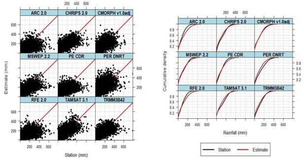
Figure 3. Monthly validation scatters plot and CDF.

Table 4. Monthly validation SREPs with gauged rainfall data over Omo River Basin from 2000-2020.

Name	ARC	CHRIPS	CMORPH	MSWEP	PE CDR	PER DNRT	RFE	TAMSAT	3B42	Perfect. Score
CORR	0.6	0.8	0.7	0.8	0.7	0.7	0.7	0.8	0.8	1
R2	0.4	0.6	0.5	0.6	0.5	0.5	0.4	0.6	0.6	1
BIAS	0.7	1.1	1.0	1.0	0.9	1.3	0.8	1.1	1.1	1
PBIAS	-27.1	8.7	-4.1	-1	-8	25.1	-17	11.7	7.2	0
ME	-32.1	10	-4.7	-1.1	-9.6	29.2	-19.9	13.6	8.5	0
MAE	59.2	43.4	47.8	41.6	49.6	59	53.3	50	45.6	0
RMSE	87.6	63.8	71.8	63.6	73.4	86.1	79.5	71.3	67.2	0
NSE	0.3	0.6	0.5	0.6	0.5	0.3	0.4	0.5	0.6	1
POD	0.9	1.0	1.0	1.0	1.0	1.0	1.0	0.9	1.0	1
POFD	0.3	0.9	0.4	0.6	0.9	0.8	0.7	0.4	0.7	0
FAR	0.0	0.1	0.0	0.0	0.1	0.1	0.0	0.0	0.0	0
CSI	0.9	0.9	0.9	0.9	0.9	0.9	0.9	0.9	1.0	1
HSS	0.5	0.1	0.6	0.5	0.2	0.3	0.4	0.4	0.4	1
VHI	0.7	1.0	0.9	0.9	0.9	1.0	0.8	1.0	1.0	1
QPOD	0.7	0.9	0.9	0.9	0.9	0.9	0.8	0.9	0.9	1
VFAR	0.1	0.1	0.1	0.1	0.1	0.2	0.1	0.1	0.1	0
QFAR	0.2	0.2	0.1	0.1	0.2	0.2	0.2	0.2	0.2	0
VMI	0.3	0.0	0.1	0.1	0.1	0.0	0.2	0.0	0.0	0
QMISS	0.3	0.1	0.1	0.1	0.1	0.1	0.2	0.1	0.1	0
VCSI	0.6	0.8	0.8	0.8	0.8	0.8	0.7	0.8	0.8	1
QCSI	0.6	0.8	0.8	0.8	0.7	0.7	0.7	0.8	0.8	1
Cat.thres.>=	1	1	1	1	1	1	1	1	1	NA
Vol.thres.value	80	80	80	80	80	80	80	80	80	NA

Download: Download full-size image

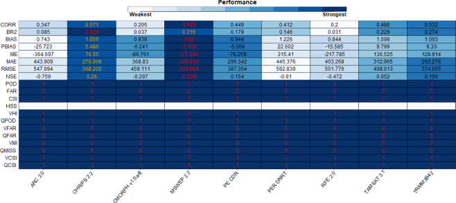
Figure 4. The overall annual validation output between SREPs and observed ground rainfall data from 2000-2020 over OR.

4.3. Analyzing Spatial Temporal Rainfall Variability

According to the overall evaluation, all SREPs have a good correlation when increasing the accumulation time series and using long-year station data, So, in this study, MSWEP was chosen to assess the spatio- temporal variability and trend of rainfall over ORB for the period of 1990–2017.

4.3.1. Rainfall Distribution

As displayed in figure 5, the overall outcome demonstrates the annual mean rainfall distribution over the entire basin, showing a range of 200–2000 mm. The greater rainfall distribution occurred in the western, central, and some parts of the north and southwest of the basin, and most probably the southern and northern parts of the basin have a lower the rainfall regime in the northern and central regions of the basin is unimodal (March to October) and bimodal (March to May) in the south. to medium rainfall distribution. The seasonal rainfall distribution, on the other hand, shows a lower rainfall amount in winter and autumn and medium and strong rainfall distribution in spring and summer. As a result, the rainfall regime in the northern and central regions of the basin is unimodal (March to October) and bimodal (March to May) in the south.

Download: Download full-size image

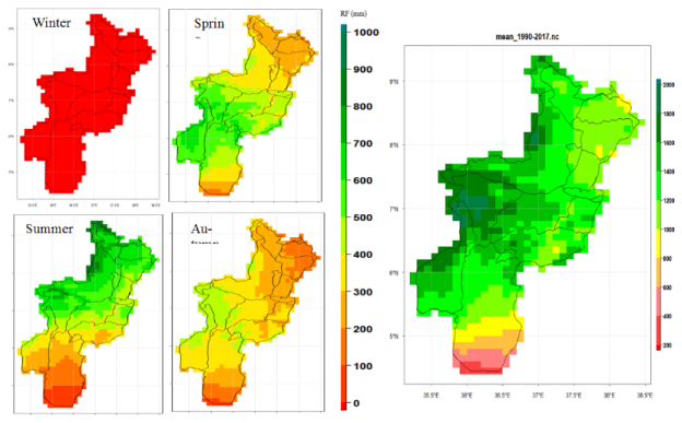
Figure 5. Annual and Seasonal spatial average rainfall distribution over ORB from 1990-2017.

4.3.2. Spatiotemporal Rainfall Variability over ORB (CV, SRA, and MK Trend Analysis)

According to Figure 6, the seasonal, and annual CV results, the basin is expressed as having low to high rainfall variation in the northern, central, western, and southern parts of basin. The basin experiences high to low variability the northern, central, western, and southern parts of the basin. The basin experiences high to low variability during the winter season, followed by autumn, spring, and summer, and low to medium variability annual.

4.3.3. Standardized Rainfall Anomaly Index (SRAI)

The inter-annual and seasonal rainfall variability over the observed time series was implied by the computation of the standard rainfall anomalies, which revealed both positive and negative anomalies. According to Figure 8, the overall inter-annual SRAI from 1990 to 2017 evaluation shows a strong positive and negative rainfall anomaly in 1997, 2006, 2015, and 1999, 2012, 2016, respectively, when compared to the remaining years. According to these results, the inter-annual rainfall variability in the Omo River basin is teleconnection to the ENSO index, and high rainfall in the basin is likely to occur during La Nia years and dry years during El Nio years. The highest positive SRAI was observed in 1997 and 2006, which exhibit very extreme wetness (> 2.5). This output, also endorsed by

[32, 33]

claimed that some of the devastating floods that occurred in August 2006 and killed 364 people and displaced over 15,000 people in 14 villages were caused by climate change and variability. While the highest negative SRAI was found in 1999 (> 2), which is extremely dry, it flowed into 2012 and 2016, which are pronounced moderately dry over the entire basin. Similar results were reported by

[34, 35]

. According to recent literature, Ethiopia has experienced twelve extreme historical droughts that have had an impact on the nation's economic growth

[36, 26]

. The occurrence of ENSO, which has had an impact on the lives of hun-dreds of thousands of indigenous people who rely on these waters for their pastoral, agro pastoral, and fishing activities, would destroy both river flow volume and lake level

[32, 37]

Download: Download full-size image

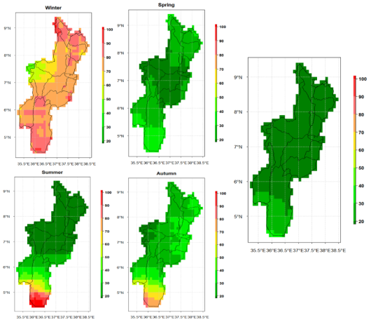
Figure 6. Spatiotemporal annual and seasonal of CV in ORB (1990-2017).

4.4. Trend Analysis

MK and Sen’s Slope

The statistical results of the MK trend test and Sen’s slope estimators for annual rainfall are given in Figure 7, the statistical monotonic upward positive trend observed in the southern, some of central, and northwestern parts of the basin. A monotonic downward negative trend was observed in the northern, some of the western and eastern parts of the basin this result was also supported by

[38]

stated at a mean annual time scale, rainfall in the Upper Omo-Gibe River showed statistically declining trends, although seasonal rainfall showed inconsistent results in both directions. However, the mean annual rainfall trend, rainfall is generally homogenous and decreasing but it was the insignificant rate in northern, western central, and some of the southern and southwest tip parts of the basin and significant in some of northeast and southern parts of the entire basin. This result agreed with

[38, 39]

in southern Ethiopia and in north-central Ethiopia. Their finding showed that decreasing RF pattern since about 1981.

Download: Download full-size image

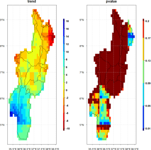
Figure 7. The overall annual MK tend analysis over ORB from 1990-2017.

Download: Download full-size image

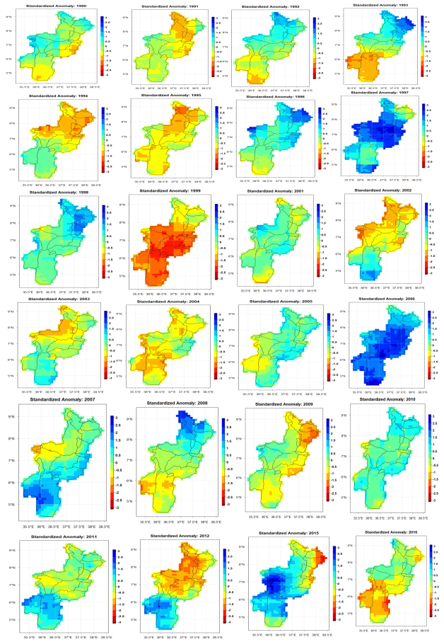
Figure 8. Annual SRAI over ORB from (1990-2017).

5. Conclusion

The overall statistical, categorical, and volumetric validation index results show that (daily, decadal, monthly, seasonal, and annual) MSWEP, CHRIPS, 3B42, and TAMSAT scored a good performance detecting capability compared to the remaining products (ARC, RFE, PER CDR, PER DNRT, and CMORPH). According to the overall evaluation, all SREPs have a good correlation when increasing the accumulation time series and using long-year station data, but a higher RMSE is observed. MSWEP, CMORPH, PERCDR RFE, and ARC have better aggregation with a slight underestimation of gauge rainfall products, whereas 3B42, CHRIPS, TAMSAT, and PER DNRT have an overestimation of rain gauge data. Furthermore, having a high spatiotemporal resolution, utilizing multiple algorithms calibrated with station data, and integrating diverse data sources is assisting more SREPs in developing their accuracy and selecting them for various applications. So, in this study, MSWEP was chosen to assess the spatio-temporal variability and trend of rainfall over ORB for the period of 1990–2017. The overall outcome demonstrates the annual mean rainfall distribution over the entire basin, showing a range of 200–2000 mm. The seasonal rainfall distribution, on the other hand, shows a lower rainfall amount in winter and autumn and medium and strong rainfall distribution in spring and summer. As a result, the rainfall regime in the northern and central regions of the basin is unimodal (March to October) and bimodal (March to May) in the south. According to monthly, seasonal, and annual CV results, the basin is expressed as having low to high rainfall variation in the northern, central, western, and southern parts of the basin. The basin experiences high to low variability during the winter season, followed by autumn, spring, and summer, and low to medium variability annually. In addition, the entire basin had a significant positive and negative rainfall anomalies index. Occasionally, these anomalies cause major floods and droughts that undoubtedly have an impact on the basin and its resources. The basin has an increasing trend from the south to the north, as shown by the annual average MK trend, and a decreasing trend in the north and the northern tip of the basin. A non- significantly decreasing trend was observed in the most of the entire basin in all seasons. As recommendation, overall, the Omo river basin is that have an area of arid and semi-arid regions, distinguished by their infrequent rainfall. Rainfall varies greatly in terms of intensity and geographic and temporal dispersion. Communities in the research region are either agro pastoral or pastoral and the very sensitive effects of climate change on these industries Drought is one of the climate extremes that commonly occur in this area and has a big impact on these populations. Extreme rainfall in this area has a number of negative repercussions, including a lack of surface and ground water, crop losses, and a lack of cattle feed. Communities and local actors must therefore develop suitable adaptation methods that will increase their abilities during and after a disaster and help them to withstand its negative impacts. The decision-makers must exercise good judgment.

Abbreviations

SREPs	Satellite Rainfall Estimation Products
USAID/(SWP)	U.S. Agency for International Development/ Sustainable Water Partnership
PMW	Passive Microwave
TIR	Thermal Infrared
CCD	Cold Cloud Duration
ORB	Omo River Basin
CDT	Climate Data Analysis Tool
STRM	Shuttle Radar Topography Mission
TAMSAT	Tropical Applications of Meteorology Using Satellite Data and Ground-Based
CHIRPS	Climate Hazards Group Infrared Precipitation with Station Data
MTSAT	Multi-Functional Transport Satellite
GOES	Geostationary Operational Environmental Satellite Network
MSWEP	Multi-Source Weighted-Ensemble Precipitation

Acknowledgments

I want to express my deepest gratitude to Ethiopian Meteorology Institute for giving this learning opportunity and providing me with meteorological data and for their thoughtfulness and special thanks to Dr. Asaminew Teshome for his kind advice and suggestion. Additionally, I would like to express my gratitude to Ethiopian Space Science and Geospatial Institute for everting.

Author Contributions

Elsabet Temesgen Asefw: Resources, Data curation, Software, Formal Analysis, Validation, Investigation, Writing - original draft, Methodology, Visualization, Project administration, Writing - review & editing

Getachew Tesfaye Ayehu: Conceptualization, Software, Formal Analysis, Supervision, Investigation, Visualization, Project administration, Writing - review & editing

Conflicts of Interest

The authors declare no conflicts of interest.

References

[1]	L. A. Al-Maliki, S. K. Al-Mamoori, I. A. Jasim, K. El-Tawel, N. Al-Ansari, and F. G. Comair, “Perception of climate change effects on water resources: Iraqi undergraduates as a case study,” Arab. J. Geosci., vol. 15, no. 6, p. 503, 2022, https://doi.org/10.1007/s12517-022-09695-y
[2]	I. Niang et al., “Africa,” Clim. Chang. 2014 Impacts, Adapt. Vulnerability Part B Reg. Asp. Work. Gr. II Contrib. to Fifth Assess. Rep. Intergov. Panel Clim. Chang., pp. 1199–1266, 2015, https://doi.org/10.1017/CBO9781107415386.002
[3]	USAID/Sustainable Water Partnership (SWP), “Ethiopia Water Resources Profile Overview,” Winrock Int., p. 11, 2021.
[4]	M. Li, “Rainfall Distribution in Ethiopia Mengying Li Columbia University,” 2014.
[5]	W. Legese, D. Koricha, and K. Ture, “Characteristics of Seasonal Rainfall and its Distribution Over Bale Highland, Southeastern Ethiopia,” J. Earth Sci. Clim. Change, vol. 09, no. 02, 2018, https://doi.org/10.4172/2157-7617.1000443
[6]	Z. T. Segele and P. J. Lamb, “Characterization and variability of Kiremt rainy season over Ethiopia,” Meteorol. Atmos. Phys., vol. 89, no. 1, pp. 153–180, 2005, https://doi.org/10.1007/s00703-005-0127-x
[7]	H. Birara, R. P. Pandey, and S. K. Mishra, “Trend and variability analysis of rainfall and temperature in the tana basin region, Ethiopia,” J. Water Clim. Chang., vol. 9, no. 3, pp. 555–569, 2018, https://doi.org/10.2166/wcc.2018.080
[8]	T. Dinku, P. Ceccato, E. Grover-Kopec, M. Lemma, S. J. Connor, and C. F. Ropelewski, “Validation of satellite rainfall products over East Africa’s complex topography,” Int. J. Remote Sens., vol. 28, no. 7, pp. 1503–1526, 2007, https://doi.org/10.1080/01431160600954688
[9]	S. Xiao, J. Xia, and L. Zou, “Evaluation of multi-satellite precipitation products and their ability in capturing the characteristics of extreme climate events over the Yangtze River Basin, China,” Water (Switzerland), vol. 12, no. 4, 2020, https://doi.org/10.3390/W12041179
[10]	M. M. Alemu and G. T. Bawoke, “Analysis of spatial variability and temporal trends of rainfall in Amhara Region, Ethiopia,” J. Water Clim. Chang., vol. 11, no. 4, pp. 1505–1520, 2020, https://doi.org/10.2166/wcc.2019.084
[11]	N. S. Sinta, A. K. Mohammed, Z. Ahmed, and R. Dambul, “Evaluation of Satellite Precipitation Estimates Over Omo–Gibe River Basin in Ethiopia,” Earth Syst. Environ., vol. 6, no. 1, pp. 263–280, 2022, https://doi.org/10.1007/s41748-021-00288-5
[12]	T. G. Romilly and M. Gebremichael, “Evaluation of satellite rainfall estimates over Ethiopian river basins,” Hydrol. Earth Syst. Sci., vol. 15, no. 5, pp. 1505–1514, 2011, https://doi.org/10.5194/hess-15-1505-2011
[13]	G. T. Ayehu, T. Tadesse, B. Gessesse, and T. Dinku, “Validation of new satellite rainfall products over the Upper Blue Nile Basin, Ethiopia,” Atmos. Meas. Tech., vol. 11, no. 4, pp. 1921–1936, 2018, https://doi.org/10.5194/amt-11-1921-2018
[14]	G. Kabite Wedajo, M. Kebede Muleta, and B. Gessesse Awoke, “Performance evaluation of multiple satellite rainfall products for Dhidhessa River Basin (DRB), Ethiopia,” Atmos. Meas. Tech., vol. 14, no. 3, pp. 2299–2316, 2021, https://doi.org/10.5194/amt-14-2299-2021
[15]	D. Fenta Mekonnen and M. Disse, “Analyzing the future climate change of Upper Blue Nile River basin using statistical downscaling techniques,” Hydrol. Earth Syst. Sci., vol. 22, no. 4, pp. 2391–2408, 2018.
[16]	D. S. Wilks, Statistical methods in the atmospheric sciences, vol. 100. Academic press, 2011.
[17]	A. Aghakouchak and A. Mehran, “Extended contingency table: Performance metrics for satellite observations and climate model simulations,” Water Resour. Res., vol. 49, no. 10, pp. 7144–7149, 2013, https://doi.org/10.1002/wrcr.20498
[18]	H. E. Beck et al., “Daily evaluation of 26 precipitation datasets using Stage-IV gauge-radar data for the CONUS,” Hydrol. Earth Syst. Sci., vol. 23, no. 1, pp. 207–224, 2019, https://doi.org/10.5194/hess-23-207-2019
[19]	Y. Kassa, “Addis Ababa Institute of Technology School of Civil and Environmental Engineering Postgraduate Program in Hydraulic Engineering,” no. November, 2013.
[20]	M. O. Kisaka, M. Mucheru-Muna, F. K. Ngetich, J. N. Mugwe, D. Mugendi, and F. Mairura, “Rainfall variability, drought characterization, and efficacy of rainfall data reconstruction: Case of Eastern Kenya,” Adv. Meteorol., vol. 2015, 2015, https://doi.org/10.1155/2015/380404
[21]	W. B. Abegaz, “Rainfall Variability and Trends over Central Ethiopia,” Int. J. Environ. Sci. Nat. Resour., vol. 24, no. 4, 2020, https://doi.org/10.19080/ijesnr.2020.24.556144
[22]	G. Bayable, G. Amare, G. Alemu, and T. Gashaw, “Spatiotemporal variability and trends of rainfall and its association with Pacific Ocean Sea surface temperature in West Harerge Zone, Eastern Ethiopia,” Environ. Syst. Res., vol. 10, no. 1, 2021, https://doi.org/10.1186/s40068-020-00216-y
[23]	C. Funk et al., “The climate hazards infrared precipitation with stations - A new environmental record for monitoring extremes,” Sci. Data, vol. 2, pp. 1–21, 2015, https://doi.org/10.1038/sdata.2015.66
[24]	J. B. et Al, “Standardized Precipitation Index User Guide,” J. Appl. Bacteriol., vol. 63, no. 3, pp. 197–200, 1987.
[25]	S. Ghaedi and A. Shojaian, “Spatial and Temporal Variability of Precipitation Concentration in Iran,” Geogr. Pannonica, vol. 24, no. 4, pp. 244–251, 2020, https://doi.org/10.5937/GP24-27361
[26]	F. A. Anose, K. T. Beketie, T. T. Zeleke, D. Y. Ayal, G. L. Feyisa, and B. T. Haile, “Spatiotemporal analysis of droughts characteristics and drivers in the Omo-Gibe River basin, Ethiopia,” Environ. Syst. Res., vol. 11, no. 1, 2022, https://doi.org/10.1186/s40068-022-00246-8
[27]	P. Nguyen et al., “Persiann dynamic infrared–rain rate (PDIR-now): A near-real-time, quasi-global satellite precipitation dataset,” J. Hydrometeorol., vol. 21, no. 12, pp. 2893–2906, 2020, https://doi.org/10.1175/JHM-D-20-0177.1
[28]	K. Teshome and F. Behulu, “Comparison of High-Resolution Satellite Based Rainfall Products at Basin Scale: The Case of Omo-Gibe River Basin, Ethiopia,” vol. 165, no. January, pp. 110–129, 2022.
[29]	A. Thesis, “Satellite-Based Rainfall Estimation: Evaluation and Characterization (A Case Study Over Omo-Gibe River Basin),” no. July, 2007.
[30]	M. Dembélé and S. J. Zwart, “Evaluation and comparison of satellite-based rainfall products in Burkina Faso, West Africa,” Int. J. Remote Sens., vol. 37, no. 17, pp. 3995–4014, 2016, https://doi.org/10.1080/01431161.2016.1207258
[31]	T. Dinku, K. Hailemariam, R. Maidment, E. Tarnavsky, and S. Connor, “Combined use of satellite estimates and rain gauge observations to generate high-quality historical rainfall time series over Ethiopia,” Int. J. Climatol., vol. 34, no. 7, pp. 2489–2504, 2014, https://doi.org/10.1002/joc.3855
[32]	M. A. Degefu and W. Bewket, “Variability and trends in rainfall amount and extreme event indices in the Omo-Ghibe River Basin, Ethiopia,” Reg. Environ. Chang., vol. 14, no. 2, pp. 799–810, 2014, https://doi.org/10.1007/s10113-013-0538-z
[33]	A. Aklilu, A., Alebachew, Assessment of climate change-induced hazards, impacts and responses in the southern lowlands of Ethiopia. Forum for Social Studies, Addis Ababa., no. 4. 2009.
[34]	N. Debela, C. Mohammed, K. Bridle, R. Corkrey, and D. McNeil, “Perception of climate change and its impact by smallholders in pastoral/agropastoral systems of Borana, South Ethiopia,” Springerplus, vol. 4, no. 1, 2015, https://doi.org/10.1186/s40064-015-1012-9
[35]	F. A. Anose, K. T. Beketie, T. Terefe Zeleke, D. Yayeh Ayal, and G. Legese Feyisa, “Spatio-temporal hydro-climate variability in Omo-Gibe River Basin, Ethiopia,” Clim. Serv., vol. 24, p. 100277, 2021, https://doi.org/10.1016/j.cliser.2021.100277
[36]	M. Taye, D. Sahlu, B. F. Zaitchik, and M. Neka, “Evaluation of satellite rainfall estimates for meteorological drought analysis over the upper blue nile basin, Ethiopia,” Geosci., vol. 10, no. 9, pp. 1–22, 2020, https://doi.org/10.3390/geosciences10090352
[37]	C. J. Carr, River Basin Development and Human Rights in Eastern Africa - A Policy Crossroads. 2017. https://doi.org/10.1007/978-3-319-50469-8
[38]	M. B. Toma, “Trend Analysis of Climatic and Hydrological Parameters in Ajora-Woybo Watershed, Omo-Gibe River Basin, Ethiopia,” 2021.
[39]	A. Asfaw, B. Simane, A. Hassen, and A. Bantider, “Variability and time series trend analysis of rainfall and temperature in northcentral Ethiopia: A case study in Woleka sub-basin,” Weather Clim. Extrem., vol. 19, no. December 2017, pp. 29–41, 2018, https://doi.org/10.1016/j.wace.2017.12.002

Cite This Article

Plain Text BibTeX RIS

APA Style

Asefw, E. T., Ayehu, G. T. (2024). Validating the Skills of Satellite Rainfall Products and Spatiotemporal Rainfall Variability Analysis over Omo River Basin in Ethiopia. Hydrology, 12(2), 36-51. https://doi.org/10.11648/j.hyd.20241202.13

Copy | Download

ACS Style

Asefw, E. T.; Ayehu, G. T. Validating the Skills of Satellite Rainfall Products and Spatiotemporal Rainfall Variability Analysis over Omo River Basin in Ethiopia. Hydrology. 2024, 12(2), 36-51. doi: 10.11648/j.hyd.20241202.13

Copy | Download

AMA Style

Asefw ET, Ayehu GT. Validating the Skills of Satellite Rainfall Products and Spatiotemporal Rainfall Variability Analysis over Omo River Basin in Ethiopia. Hydrology. 2024;12(2):36-51. doi: 10.11648/j.hyd.20241202.13

Copy | Download

@article{10.11648/j.hyd.20241202.13,
  author = {Elsabet Temesgen Asefw and Getachew Tesfaye Ayehu},
  title = {Validating the Skills of Satellite Rainfall Products and Spatiotemporal Rainfall Variability Analysis over Omo River Basin in Ethiopia
},
  journal = {Hydrology},
  volume = {12},
  number = {2},
  pages = {36-51},
  doi = {10.11648/j.hyd.20241202.13},
  url = {https://doi.org/10.11648/j.hyd.20241202.13},
  eprint = {https://article.sciencepublishinggroup.com/pdf/10.11648.j.hyd.20241202.13},
  abstract = {Recently created long-term and regionally dispersed satellite-based rainfall estimates have emerged as crucial sources of rainfall data to assess rainfall's spatial and temporal variability, particularly for data-scarce locations. Objective (the general): The purpose of this paper is to assess the skills of nine selected satellite rainfall estimates i.e., (ARC 2.0, TRMM 3B42, CHIRPS v. 2.0, TAMSAT 3.1, CMORPH v. 1.0 adj., PERSIANN CDR and DNRT, and MSWEP v. 2.2) and understand Spatio-temporal variability of rainfall over the Omo River basin using the best performing product. Method: The validation analysis was done by using a point-to-grid-based comparison test at different temporal accumulations. MSWEP was selected as the best product to analyze the long-term trend and variability of rainfall over the Omo-River basin from 1990-2017. The coefficients of variation (CV) and the standardization rainfall anomalies index (SRAI) were used to examine rainfall variability, while the Mann-Kendall (MK) and Sen slope estimators were used to examine the trend and magnitude of rainfall patterns. Results: The overall statistical, categorical, and volumetric validation index results show that the MSWEP is the best performing rainfall product followed by CHRIPS, 3B42, and TAMSAT according to their order of appearance than the remaining products (i.e., ARC, RFE, PER CDR, PER DNRT, and CMORPH). The CV result with the relatively highest monthly variability (CV > 30%) was observed in some southern, northern, southeastern, and central parts of the study area. In general, the overall annual CV shows almost no variation in the entire basin except in the lower part because of the region's prevalent topographic variances, which ranged from 3455 to 352 m.a.s.l. In addition, the highest seasonal positive and negative anomalies are observed in each season in the entire basin. These abnormalities can result in significant floods and droughts that unquestionably influence the basin and its resources. Conclusion: In general, the basin has an increasing trend in the southern portions and a declining trend in the central to northern tip parts of the basin, as can be observed from the annual average MK trend tests. The basin has experienced a greeter variation but is not significant except in some parts of the basin.
},
 year = {2024}
}

Copy | Download

TY - JOUR
T1 - Validating the Skills of Satellite Rainfall Products and Spatiotemporal Rainfall Variability Analysis over Omo River Basin in Ethiopia

AU - Elsabet Temesgen Asefw
AU - Getachew Tesfaye Ayehu
Y1 - 2024/06/29
PY - 2024
N1 - https://doi.org/10.11648/j.hyd.20241202.13
DO - 10.11648/j.hyd.20241202.13
T2 - Hydrology
JF - Hydrology
JO - Hydrology
SP - 36
EP - 51
PB - Science Publishing Group
SN - 2330-7617
UR - https://doi.org/10.11648/j.hyd.20241202.13
AB - Recently created long-term and regionally dispersed satellite-based rainfall estimates have emerged as crucial sources of rainfall data to assess rainfall's spatial and temporal variability, particularly for data-scarce locations. Objective (the general): The purpose of this paper is to assess the skills of nine selected satellite rainfall estimates i.e., (ARC 2.0, TRMM 3B42, CHIRPS v. 2.0, TAMSAT 3.1, CMORPH v. 1.0 adj., PERSIANN CDR and DNRT, and MSWEP v. 2.2) and understand Spatio-temporal variability of rainfall over the Omo River basin using the best performing product. Method: The validation analysis was done by using a point-to-grid-based comparison test at different temporal accumulations. MSWEP was selected as the best product to analyze the long-term trend and variability of rainfall over the Omo-River basin from 1990-2017. The coefficients of variation (CV) and the standardization rainfall anomalies index (SRAI) were used to examine rainfall variability, while the Mann-Kendall (MK) and Sen slope estimators were used to examine the trend and magnitude of rainfall patterns. Results: The overall statistical, categorical, and volumetric validation index results show that the MSWEP is the best performing rainfall product followed by CHRIPS, 3B42, and TAMSAT according to their order of appearance than the remaining products (i.e., ARC, RFE, PER CDR, PER DNRT, and CMORPH). The CV result with the relatively highest monthly variability (CV > 30%) was observed in some southern, northern, southeastern, and central parts of the study area. In general, the overall annual CV shows almost no variation in the entire basin except in the lower part because of the region's prevalent topographic variances, which ranged from 3455 to 352 m.a.s.l. In addition, the highest seasonal positive and negative anomalies are observed in each season in the entire basin. These abnormalities can result in significant floods and droughts that unquestionably influence the basin and its resources. Conclusion: In general, the basin has an increasing trend in the southern portions and a declining trend in the central to northern tip parts of the basin, as can be observed from the annual average MK trend tests. The basin has experienced a greeter variation but is not significant except in some parts of the basin.

VL - 12
IS - 2
ER -

Copy | Download

Author Information

Elsabet Temesgen Asefw

Ethiopia Meteorological Institute, Addis Ababa, Ethiopia; Remote Sensing Research and Development Department, Entoto Obsrbatory Research Centre, Ethiopian Space Science and Geospatial Institute, Addis Ababa, Ethiopia

Contact Email

http://orcid.org/0009-0007-8520-625X
Getachew Tesfaye Ayehu

Alliance of Bioversity and CIAT, Addis Ababa, Ethiopia

Contact Email

Download PDF

Plain Text BibTeX RIS

APA Style

Asefw, E. T., Ayehu, G. T. (2024). Validating the Skills of Satellite Rainfall Products and Spatiotemporal Rainfall Variability Analysis over Omo River Basin in Ethiopia. Hydrology, 12(2), 36-51. https://doi.org/10.11648/j.hyd.20241202.13

Copy | Download

ACS Style

Asefw, E. T.; Ayehu, G. T. Validating the Skills of Satellite Rainfall Products and Spatiotemporal Rainfall Variability Analysis over Omo River Basin in Ethiopia. Hydrology. 2024, 12(2), 36-51. doi: 10.11648/j.hyd.20241202.13

Copy | Download

AMA Style

Asefw ET, Ayehu GT. Validating the Skills of Satellite Rainfall Products and Spatiotemporal Rainfall Variability Analysis over Omo River Basin in Ethiopia. Hydrology. 2024;12(2):36-51. doi: 10.11648/j.hyd.20241202.13

Copy | Download

@article{10.11648/j.hyd.20241202.13,
  author = {Elsabet Temesgen Asefw and Getachew Tesfaye Ayehu},
  title = {Validating the Skills of Satellite Rainfall Products and Spatiotemporal Rainfall Variability Analysis over Omo River Basin in Ethiopia
},
  journal = {Hydrology},
  volume = {12},
  number = {2},
  pages = {36-51},
  doi = {10.11648/j.hyd.20241202.13},
  url = {https://doi.org/10.11648/j.hyd.20241202.13},
  eprint = {https://article.sciencepublishinggroup.com/pdf/10.11648.j.hyd.20241202.13},
  abstract = {Recently created long-term and regionally dispersed satellite-based rainfall estimates have emerged as crucial sources of rainfall data to assess rainfall's spatial and temporal variability, particularly for data-scarce locations. Objective (the general): The purpose of this paper is to assess the skills of nine selected satellite rainfall estimates i.e., (ARC 2.0, TRMM 3B42, CHIRPS v. 2.0, TAMSAT 3.1, CMORPH v. 1.0 adj., PERSIANN CDR and DNRT, and MSWEP v. 2.2) and understand Spatio-temporal variability of rainfall over the Omo River basin using the best performing product. Method: The validation analysis was done by using a point-to-grid-based comparison test at different temporal accumulations. MSWEP was selected as the best product to analyze the long-term trend and variability of rainfall over the Omo-River basin from 1990-2017. The coefficients of variation (CV) and the standardization rainfall anomalies index (SRAI) were used to examine rainfall variability, while the Mann-Kendall (MK) and Sen slope estimators were used to examine the trend and magnitude of rainfall patterns. Results: The overall statistical, categorical, and volumetric validation index results show that the MSWEP is the best performing rainfall product followed by CHRIPS, 3B42, and TAMSAT according to their order of appearance than the remaining products (i.e., ARC, RFE, PER CDR, PER DNRT, and CMORPH). The CV result with the relatively highest monthly variability (CV > 30%) was observed in some southern, northern, southeastern, and central parts of the study area. In general, the overall annual CV shows almost no variation in the entire basin except in the lower part because of the region's prevalent topographic variances, which ranged from 3455 to 352 m.a.s.l. In addition, the highest seasonal positive and negative anomalies are observed in each season in the entire basin. These abnormalities can result in significant floods and droughts that unquestionably influence the basin and its resources. Conclusion: In general, the basin has an increasing trend in the southern portions and a declining trend in the central to northern tip parts of the basin, as can be observed from the annual average MK trend tests. The basin has experienced a greeter variation but is not significant except in some parts of the basin.
},
 year = {2024}
}

Copy | Download

TY - JOUR
T1 - Validating the Skills of Satellite Rainfall Products and Spatiotemporal Rainfall Variability Analysis over Omo River Basin in Ethiopia

VL - 12
IS - 2
ER -

Copy | Download