Comparative Performance of Non-Stationary Intensity-Duration-Frequency (NS-IDF) Models for Selected Gauge Stations in the Niger Delta

Masi Gabriel Sam; Ify Lawrence Nwaogazie

doi:doi:10.11648/j.hyd.20241202.11

Research Article |

| Peer-Reviewed

Comparative Performance of Non-Stationary Intensity-Duration-Frequency (NS-IDF) Models for Selected Gauge Stations in the Niger Delta

Masi Gabriel Sam

, Ify Lawrence Nwaogazie^*

Published in Hydrology (Volume 12, Issue 2)

Received: 27 April 2024 Accepted: 20 May 2024 Published: 6 June 2024

Views: Downloads:

Download PDF

Share This Article

Twitter
Linked In
Facebook

Abstract

This study focused on a comparative analysis of developed Non-stationary rainfall intensity-duration-frequency (NS-IDF) models with existing IDF models for the Niger Delta with Uyo, Benin, Port Harcourt, and Warri as selected stations. Applied was 24-hourly (daily) annual maximum series (AMS) data with downscaling models also used to downscale the time series data. Uyo and Benin had statistically significant trends with Port Harcourt and Warri showing mild trends. The best linear behavioural parameter extremes model integrating time as co-variate was selected for each station for computation of the General extreme value (GEV) distribution fitted NS-IDF models with the open-access R-studio software. The Non-stationary intensity values were higher than computed stationary ones, with significant differences at a 5% significance level for a given return period. For example, for 2 and 10-year return periods for 1-hour storms the differences of 22.71% & 17.0%, 15.24% & 9.40%, 5.09% & 4.04%, and 6.15% & 4.43% for Uyo, Benin, Port Harcourt and Warri, respectively were recorded. While, the percentage difference in intensities was very high between the Non-stationary and existing, Stationary IDF models. For a return period of 2 years at 15 and 60 min durations, the differences were 97.9 & 3.2%, 240.6 & 67.2%, 78.2 & 0%, and 121.6 & 50.1% for Uyo, Benin, Port Harcourt and Warri, respectively. Such extreme value difference in intensity underestimates the peak flood and exagerate the flood risk. The general NS-IDF calibrated models showed very good match and fit with R² = 0.977, 0.999, 0.999 & 0.999, and MSE accuracy = 193.5, 1.011, 4.1552 & 1.011 for Uyo, Benin, Port Harcourt, and Warri, respectively. Erosion and flood control facilities in the Niger Delta require upgrading using the calibrated general NS-IDF models to accommodate extra-value rainfall intensities due to climate change.

Published in	Hydrology (Volume 12, Issue 2)
DOI	10.11648/j.hyd.20241202.11
Page(s)	17-31
Creative Commons	This is an Open Access article, distributed under the terms of the Creative Commons Attribution 4.0 International License (http://creativecommons.org/licenses/by/4.0/), which permits unrestricted use, distribution and reproduction in any medium or format, provided the original work is properly cited.
Copyright	Copyright © The Author(s), 2024. Published by Science Publishing Group

Keywords

Rainfall, Annual Maximum Series, Stationary, Non-Stationary, Curve Fitting, Modelling

1. Introduction

In hydrological designs, storm water are calculated through the mathematical formulation of the rainfall intensity-duration frequency (IDF) relationship. Most infrastructural designs are executed on the so-called Stationary assumption of the rainfall IDF relationship which is site-specific to the frequency analysis of the rainfall data, for different durations. These relationships are unreliable and often inaccurate because they are based on many assumptions such as distribution selection for each duration, and also require a large number of parameters that are dependent on time

[1]

However, Non-stationary IDF modelling introduces time series data which are sequential and dynamic to give way for the introduction of the sample means, variance, and covariance changes over time for evaluation of location parameters when a significant trend has been established

[1-4]

. Studies also confirmed that the Non-stationary IDF modelling produces more efficient and accurate estimates in the simple scaling process of rainfall IDF relationship than the Stationary method

[2]

. Further studies on IDF modelling also proved that the Non-stationary framework results in a better fit to the sample data than the Stationary approach

[5, 6]

The purpose of this study is to carry out a comparative performance study of the Non-stationary IDF models developed against the existing IDF rainfall models for the four selected meteorological gauge stations in the Niger Delta in Nigeria. The 24-hourly Annual Maximum Series (AMS) time series data were adopted for the study using different statistical approaches.

2. Methodology

2.1. Study Area

The study area is located between longitude 4^o15’N – 6^o30’N and latitudes 5^o32’E – 8^o22’E at the South of the Niger River in Nigeria. The map of the study area is presented in Figure 1 with the selected four locations GIS as follows; Uyo: 5.0377⁰N and 7.9128⁰E, Benin City: 6.3350⁰N and 5.6037⁰E, Port Harcourt: 4.8156⁰N and 7.0498⁰E, and Warri: 5.5544⁰N and 5.7932⁰E.

Heavy seasonal rainfall is experienced between March and October with a dry period having occasional rainfall occurring from November to February. The duration and intensity of the rain increase from the North to the South. The climate is further influenced by two air masses which are the South-Westerly wind laden with moisture emanating from the Atlantic Ocean, and the North-East Trade wind inducing Harmattan which follows the pattern and the duration of the Indian Monsoon wind

[7, 8]

. Thus, maintaining relatively high temperature and humidity all year round.

Download: Download full-size image

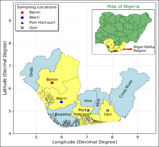
Figure 1. Map showing study stations in the Niger Delta.

2.2. Data Collection

2.2.1. Constructing Downscaled Non-Stationary Predicted Rainfall Intensities

Rainfall time series data were collected for each of the four meteorological gauge stations namely Uyo, Benin, Port Harcourt, and Warri from the Nigerian Meteorological Agency (NIMET). The period covered 30 years for Uyo, 36 years for Benin and Warri, and 35 years for Port Harcourt. The data were sorted into 24-hourly Annual Maximum Series (AMS) and desegregated into shorter durations of 0.25, 0.5, 0.75, 1, 2, 6, and 12 hours using the Indian Meteorological Department (IMD)

[9]

, and the Modified Chowdhury IMD (MCIMD)

[10]

downscaling models as demonstrated in

[11]

2.2.2. Constructing CAMS-Based PDF Computed Rainfall Intensities

Also, data were sorted out for constructing the conventional annual maximum series (CAMS) based Gumbel Extreme Value Type 1 (GEVT-1) probability distribution function (PDF) computed rainfall IDF models, replicated after Nwaogazie et al.

[12]

to serve as an existing rainfall intensity record. The data were sorted out into durations of 15, 30, 45, 60, 90, 120, 180, and 300 minutes for each year covering the years of rainfall data collection for each station. The rainfall averages for each duration were further ranked in decreasing order of magnitude for each year. The rainfall amount was divided by their corresponding duration to obtain their values in rainfall intensities (mm/hr).

2.3. Development and Application of General Extreme Value (GEV) Distribution Function Rainfall Curve Fitting

The basic steps required to follow for the development of a 24-hour GEV distribution function Curve fitting for both stationary and Non-stationary rainfall intensity are well cataloged in our earlier publications

[13, 14]

. The procedure required are as follows:-

i. Check for climatic trends in collected time series data;

ii. Fitting stationary and Non-stationary IDF Curves with GEV distribution function given as Equation (1);

F(x) = exp

[- {(1 + ξ (t) \frac{x - μ (t)}{σ (t)})}^{\frac{- 1}{ξ (t)}}]

for

ξ \neq

0(1)

where F(x) = Cumulative Distribution Function,

ξ

= shape parameter,

μ

= mean and

σ

= standard deviation.

iii. Evaluation of the GEV time-variant parameters models and selection of the best model;

iv. Deriving stationary and Non-stationary IDF Curves from Equation (2);

x_{T}

μ (t)

\frac{σ (t)}{ξ (t)} [1 - \{{- \ln (1 - \frac{1}{T})}^{- ξ (t)}\}]

for

ξ \neq

0(2)

where

x_{T}

= rainfall intensity exceedance value, and T = return period. Also, the return levels are similarly translated into intensities for each return period and duration, with IDF curves plotted.

v. Comparison of Non-stationary and stationary predicted rainfall intensities.

2.4. Calibrating Computed Rainfall Curves into Modified Sherman Equations

The modified Sherman equation given in Equation (3) was used for calibration of the general PDF-IDF models applied in obtaining the different computed rainfall intensity curves;

RainfallIntensity,

I = \frac{C T_{r}^{m}}{{T_{d}}^{a}}

(3)

where; Tr = return period (years); T_d= duration of rainfall in minutes and I = rainfall intensities (mm/hr); while c, a, and m are the physiographic constants of the catchment area.

The calibration of the general PDF-IDF model entails the inputting of 48 data sets, ie, the values of all the durations and their corresponding intensity for 6 return periods selected into Equation (3),

[11]

. Also, the calibration of the modified Sherman Equation (3), the evaluation of the mean squared error (MSE), and the coefficient of determination (R²) followed the optimization method in the literature

[15]

3. Results

3.1. Fitting Generalized Extreme Value Distribution Non-Stationary IDF Curves

The rainfall curves for the NS-IDF models were developed with the aid of the open-access software provided by the RStudio Team

[16]

. The extreme intensity values were computed based on the General extreme value (GEV) distribution with the family of three combinations of Gumbel, Frechet, and Weibull distributions. The cumulative distribution function (CDF) of the general extreme value given in Equation (1) was the basis for obtaining the log-likelihood function. Thus, by formulating the expression in the equation, it enabled the optimization of the log-likelihood function which allowed for the extension of the Non-stationarity concept, where the parameters of the GEV distributions depend on time, t. By inversion of the GEV Equation (1) produced Equation (2) used for the computation of the rainfall intensity values. However, to evaluate the parameters of the external distribution of the GEV function, this was actualized by minimizing the negative likelihood function through an iterative numerical approach.

3.2. Evaluation of GEV Parameters for Non-Stationary IDF Modeling

Non-stationarity was introduced by integrating any one selected linear parameter models into the log-likelihood function formula on the satisfaction of the shape function condition. The resulting solutions and the performances of the different statistical parameters expressed as a function of time with their values for the various stations are presented in Table 1.

Table 1. Evaluation of performance of GEV parameters used for Non-stationary and Stationary models for the various stations.

Station	Time (mins)	Models	Location Parameter	Scale	Shape Parameter	AIC	AIC_c
Uyo	15	GEV_t– 0	165.13	33.101	0.0367	311.938	312.861
		GEV_t– I	130.580 + 2.606t	32.203	-0.1354	305.853	307.453
		GEV_t– II	159.0525	14.289 + 1.510t	-0.2245	308.123	309.723
		GEV_t- III	140.637 + 1.981t	17.285 + 0.926t	-0.1848	303.691	306.191
	60	GEV_t– 0	56.031	11.731	0.0378	249.737	250.660
		GEV_t– I	43.784 + 0.924t	11.435	-0.1351	243.68	245.280
		GEV_t– II	53.8771	5.053 + 0.537t	-0.2244	245.939	247.539
		GEV_t- III	47.371 + 0.701t	6.122 + 0.329t	-0.1842	241.51	244.010
	1440	GEV_t– 0	4.8917	1.08	0.0462	106.897	107.820
		GEV_t– I	3.783 + 0.084t	1.058	-0.1293	101.153	102.753
		GEV_t– II	4.7029	0.476 + 0.049t	-0.216	103.3	104.900
		GEV_t- III	4.100 + 0.064t	0.570 + 0.030t	-0.1764	98.997	101.497
Benin	15	GEV_t– 0	146.178	35.22	0.0304	376.74	377.49
		GEV_t– I	118.019 + 1.495t	28.11	0.1722	369.01	370.30
		GEV_t– II	149.704	45.231 – 0.653t	0.1842	377.13	378.42
		GEV_t- III	117.743 + 1.511t	27.785 + 0.0194t	0.1718	371.011	373.01
	60	GEV_t– 0	49.345	12.487	0.0305	302.036	302.79
		GEV_t– I	39.405 + 0527t	9.971	0.172	294.33	295.62
		GEV_t– II	50.6118	16.074 - 0.233t	0.185	302.429	303.72
		GEV_t- III	39.293 + 0.534t	9.849 + 0.0066t	0.1719	296.327	298.33
	1440	GEV_t– 0	4.268	1.173	0.0269	131.606	132.36
		GEV_t– I	3.331 + 0.0497t	0.9358	0.168	123.911	125.20
		GEV_t– II	4.387	1.5078 - 0.022t	0.1796	132.016	133.31
		GEV_t- III	3324 + 0.0501t	0.9304 + 0.0004t	0.1664	125.99	127.99
Port Harcourt	15	GEV_t– 0	144.677	28.986	0.0666	355.21	355.98
		GEV_t– I	135.578 + 0.484t	27.878	0.1061	356.08	357.41
		GEV_t– II	144.671	30.827 - 0.126t	0.0971	357.1	358.43
		GEV_t- III	135.058 + 0.516t	27.264 + 0.040t	0.1038	358.06	360.13
	60	GEV_t– 0	48.78	10.288	0.066	282.65	283.43
		GEV_t– I	45.549 + 0.172t	9.904	0.1053	283.52	284.86
		GEV_t– II	48.771	10.935 - 0.045t	0.0969	284.54	285.87
		GEV_t- III	45.370 + 0.1873t	9.635 + 0.015t	0.1038	285.51	287.58
	1440	GEV_t– 0	4.234	0.963	0.0502	116.22	117.00
		GEV_t– I	3.924 + 0.016t	0.924	0.0944	117.07	118.40
		GEV_t– II	4.231	1.028 - 0.005t	0.0878	118.09	119.42
		GEV_t- III	3.914 + 0.017t	0.909 + 0.001t	0.0931	119.06	121.13
Warri	15	GEV_t– 0	171.381	22.944	-0.232	335.975	336.725
		GEV_t– I	161.270 + 0.582t	22.571	-0.2592	335.678	336.968
		GEV_t– II	170.475	16.435 + 0.402t	-0.2915	336.851	338.141
		GEV_t- III	162.813 + 0.508t	18.857 + 0.210t	-0.2756	337.281	339.281
	60	GEV_t– 0	58.28	8.134	-0.2325	261.268	262.018
		GEV_t– I	54.651 + 0.206t	7.993	-0.2584	260.96	262.25
		GEV_t– II	57.939	5.824 + 0.142t	-0.292	262.147	263.437
		GEV_t- III	55.161 + 0.183t	6.682 + 0.074t	-0.275	262.568	264.568
	1440	GEV_t– 0	5.112	0.747	-0.2391	89.118	89.868
		GEV_t– I	4.777 + 0.019t	0.733	-0.2641	88.704	89.9943
		GEV_t– II	5.08	0.536 + 0.013t	-0.3009	90.027	91.3173
		GEV_t- III	4.817 + 0.017t	0.622 + 0.006t	-0.2812	90.369	92.369

The best behavioral parameter extreme model was selected based on the corrected Akaike Information Criteria (AICc)

[13, 14]

. The model that had the lowest AICc was selected as the model that best represents the time series data. The values of rainfall intensities were accordingly computed for the Non-Stationary IDF curves based on the best model-selected calculated parameter values.

3.3. Computation of Non-Stationary Model Rainfall Intensities and Return Periods

The GEV distribution fitted IDF models computed rainfall intensities performed using Equation (3) for Stationary and modified for Non-stationary models, which were represented in a table for plotting. Furthermore, Figures 2 to 5 show the graphical plots of GEV distribution fitted Non-Stationary and Stationary IDF curves on a normal-graph paper for given return periods for the various stations.

3.4. Comparative Analysis of Developed GEV-Fitted Non-Stationary and Stationary IDF Models

A comparative study of differences between the GEV-fitted Non-stationary and stationary IDF model predicted rainfall intensity is hereby presented. The discussion is based on the percentage differences confirmed with the paired Wilcoxon sample non-parametric test of significance at a 95% confidence interval.

Visually perusing through the rainfall intensity distributions in Figures 2 to 5 of the graphical plots of intensity against duration is indicative of differences between the Non-stationary and the stationary models at each plotting point. Therefore, verifying if the differences were indeed.

Download: Download full-size image

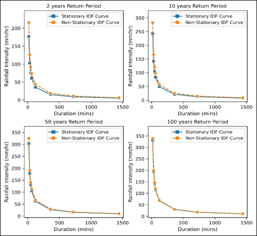
Figure 2. GEV fitted non-stationary & stationary IDF curves for the given return period for Uyo.

Download: Download full-size image

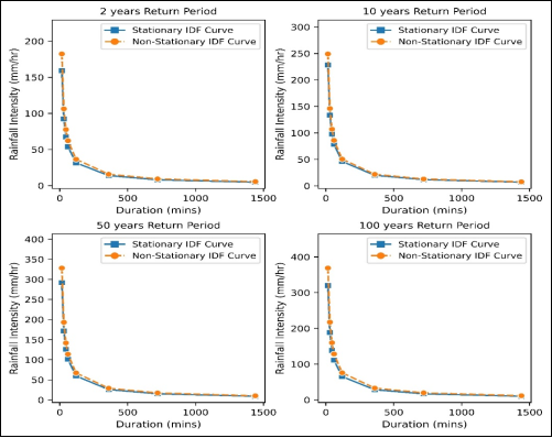
Figure 3. GEV fitted non-stationary & stationary IDF curves for given return period for Benin.

Download: Download full-size image

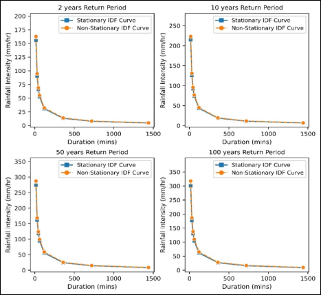
Figure 4. GEV fitted non-stationary & stationary IDF curves for given return period for Port –Harcourt.

Download: Download full-size image

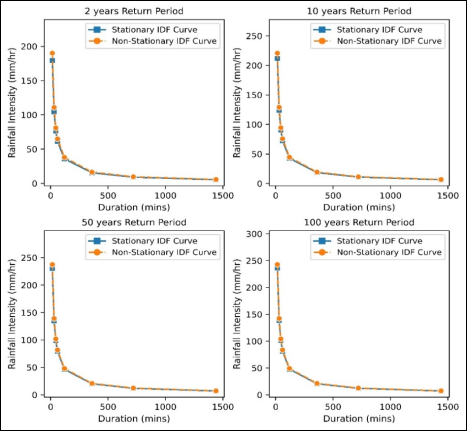
Figure 5. GEV fitted non-stationary & stationary IDF curves for given return period for Warri.

Table 2. Percentage difference of rainfall intensities between GEV fitted non-stationary and stationary IDF models for different stations.

State	Duration (mins)	Return Period (years)
State	Duration (mins)	2	5	10	25	50	100
Uyo	15	21.81^±	19.85	16.57	11.31	7.01	2.61
	30	22.27	20.20	16.82	11.46	7.08	2.62
	60	22.71	20.51	17.06	11.59	7.16	2.64
	120	23.06	20.79	17.23	11.75	7.28	2.73
	1440	23.81	21.31	17.31	11.84	7.20	2.30
Benin	15	14.65^±	9.85	9.15	10.31	12.37	15.30
	30	15.04	10.08	9.36	10.53	12.60	15.57
	60	15.24	10.14	9.40	10.55	12.64	15.62
	120	15.53	10.36	9.54	10.67	12.75	16.06
	1440	16.38	10.89	9.87	10.87	13.09	16.08
Port Harcourt	15	4.82^±	3.88	3.87	4.30	4.90	5.69
	30	4.97	4.02	3.97	4.40	4.99	5.78
	60	5.09	4.09	4.04	4.46	5.06	5.86
	120	5.29	4.19	4.15	4.55	5.15	5.95
	1440	5.44	4.01	4.29	4.88	5.72	6.51
Warri	15	5.94^±	4.89	4.29	3.62	3.18	2.78
	30	6.03	4.96	4.35	3.67	3.24	2.85
	60	6.15	5.04	4.43	3.74	3.30	2.89
	120	6.22	5.12	4.48	3.77	3.35	2.93
	1440	6.52	5.29	4.68	3.98	3.57	3.05

± Percentage Difference of Rainfall Intensities

significant is necessary and imperative. The percentage difference between the Non-stationary and Stationary intensities against duration shown in Figures 2 to 5 for the various study stations was computed and presented in Table 2. The Wilcoxon non-parametric paired test was used to verify if the percentage differences noted were statistically significant at the 95% Confidence interval. Consequently, conducted was two-tailed statistic test for rainfall intensities versus duration for a given return period. The Wilcoxon test statistic was computed and compared against the critical p-value at an alpha value of 5%.

3.5. Comparative Analysis for GEV Fitted Non-Stationary and Existing CAMS IDF Model Predicted Intensities

The objectives of this aspect of the study was to further investigate the degree of percentage differences between the Non-stationary GEV-fitted IDF curves and those of existing stationary PDF-IDF fitted curves for the study area. For this reason, the existing conventional annual maximum series (CAMS) GEVT-1 PDF computed rainfall intensities for the study area were sourced from Nwaogazie et al.

[12]

in the literature as presented. The general GEVT-1 PDF-IDF models were used to generate predicted rainfall intensities for each station. The intensity values for Non-stationary and Existing IDF models were both plotted against a corresponding duration of not more than 2 hours for different return periods for the various stations.

Download: Download full-size image

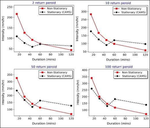
Figure 6. GEV Fitted Non-stationary and existing CAMS predicted IDF curves at 2-hr duration for Uyo.

Download: Download full-size image

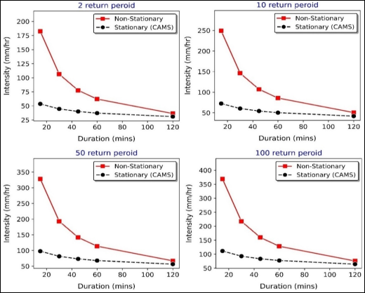
Figure 7. GEV Fitted Non-stationary and existing CAMS predicted IDF curves at 2-hr duration for Benin.

Download: Download full-size image

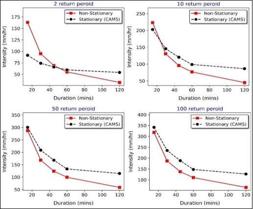
Figure 8. GEV Fitted Non-stationary and existing CAMS predicted IDF curves at 2-hr duration for Port Harcourt.

Download: Download full-size image

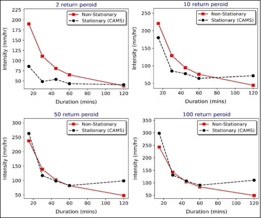
Figure 9. GEV Fitted Non-stationary and existing CAMS predicted IDF curves at 2-hr duration for Warri.

Thus, graphical plots of GEV fitted Non-stationary and existing CAMS predicted IDF curve distributions at not more than 2 hours for the various stations are presented in Figures 6 to 9 with the percentage differences computed.

3.6. Calibration of General Non-Stationary IDF (GNS-IDF) Models

The Non-stationary rainfall intensities computed were calibrated into the selected modified Sherman quotient-power empirical formula in Equation (3). Calibration was by optimization carried out with Microsoft Excel Solver of the empirical formula, the mean square error (MSE), and the coefficient of determination (R²) to obtain the general IDF model for the GEV fitted NS-IDF rainfall intensity curves for the various study stations presented in Table 3.

Table 3. Summary of GEV fitted General Non-stationary IDF (GNS-IDF) models for various stations.

Stations	IDF Models	R²	MSE
Uyo	I = $\frac{2445.37 T_{r}^{0.1065}}{T_{d}^{0.8898}}$	0.977	193.5
Benin	I = $\frac{1300.08 T_{r}^{0.1777}}{T_{d}^{0.7650}}$	0.999	1.011
Port Harcourt	I = $\frac{1160.59 T_{r}^{0.1621}}{T_{d}^{0.7686}}$	0.999	4.1552
Warri	I = $\frac{1432.20 T_{r}^{0.066}}{T_{d}^{0.771}}$	0.999	1.011

4. Discussion

4.1. Development of Non-Stationary IDF Models

The development of NS-IDF models is the derivation of IDF models, which have time-variant parameters integrated as co-variate. The statistical parameters such as mean (location), standard deviation (scale), and the shape function of the time series data are not assumed constant or uniform. The following section presents the analyses of the results of the NS-IDF modeling developed for the study area which commenced with the downscaling of the time series collected data.

The measured rainfall annual maximum time series data used in this analysis was the 24-hourly time series data with the Modified Chowdhury Indian Meteorological Department (MCIMD) downscaling model applied to generate the time series data for the analysis

[13, 14]

. In developing the Non-stationary IDF models, preference was placed on the MCIMD model downscaled time series data over others for the reason that the calibrated MCIMD model produced higher predicted rainfall intensities than the Indian Meteorological Department (IMD) method. Also, various shorter durations of 0.25 to 1.0 hours are applicable for typical urban drainage designs, and 2 to 24 hours longer durations are adequate for rural or large-scale infrastructural designs, respectively.

4.2. Significant Trend Check on Annual Maximum Time Series Data

The Mann-Kendal (MK) non-parametric and the Sen Slope estimator; were used to check for statistically significant Non-stationary behavior of the time series data

[17]

. This was to help examine the effect of ignoring non-stationarity in the 24-hour time series data collected for each station. In the results of the MK and Sen’s Slope tests earlier presented in

[18]

, a trend in the time series data was observed for each of the study stations. Therefore, the Non-stationary behaviour exhibited by the time series data for different durations in each station by showing a positive trend validates the application of Non-stationarity for the IDF modeling - an indication of evidence of changing climatic conditions.

4.3. GEV Distribution Fitted Non-Stationary IDF Curves

The computations made to obtain the rainfall IDF curves fitted based on GEV distribution were by the R-studio software. The basic equation that provided the formula for the cumulative distribution function for the GEV distribution has a family of three distribution functions controlled by the shape function for when it is zero, more than zero, or less than zero, as given by Equation (1). The expression of the equation into its log-likelihood provided the basis for computing the parameters of the GEV distribution functions for both stationary and the extension of the principles to the Non-stationary modeling when time is a co-variate. The model parameters were analyzed by optimization, which required the minimization of the negative log-likelihood obtained through an iterative process.

Four different linear models that integrate time as co-variate were selected, as shown in Table 1, for the computation of the GEV distribution function parameters. The first model, GEVt – 0, applies at constant values of location, scale, and shape parameters which is equivalent to the stationary assumption of the GEVT-1. The second model, GEVt – I had time as a co-variate with location as a parameter while scale and shape parameters were kept constant. The third model, GEVt – II has time as a co-variate with scale parameter, while location and shape parameters were kept constant. The fourth model, GEVt – III has only the shape parameter constant while time serves as a co-variate with both locations and scale parameters.

4.4. Selection Process for Best Parameter Models

Having computed the GEV distribution function parameter function for each linear model, the next step is to select the best-performing linear model. The statistical method used was based on Corrected Akaike Information Criteria (AIC_C). The model with the least AIC_C was considered a reasonable and good choice. For instance, for Uyo, the GEVt – III from Table 1, which had time as co-variate with both location and scale parameters while the shape parameter as constant gave the least AIC_C for all durations analyzed. Thus, for Uyo the fourth model, GEVt – III, was selected as the best parameter model used for the computation of the Non-stationary rainfall intensities for the different return periods of 2, 5, 10, 25, 50, and 100 years. For other stations, such as Benin, the best linear model was model type 2 (GEVt – I) from Table 1, with the least AIC_C for all durations and had 370.3 and 125.20 values for 15 min and 1440 min durations, respectively.

Also, the Port Harcourt station had its best linear model as model type 1 (GEVt – 0) with least AIC_C of 355.98 and 117.0 for 15 min and 1440 min durations, respectively. This model is the stationary type equivalent to the Gumbel Extreme Value Type-1 (GEVT-1) model. This outcome implies that time does not influence the parameter models confirming no significant trend in the rainfall time series data. In this case, the time-series data is a uniformly distributed rainfall pattern.

The AIC_C results for Warri are similar to those of Port Harcourt where the best AIC_C results were 336.725 and 89.868 for 15 min and 1440 min durations, respectively; produced from the GEV fitted stationary model type 1 (GEVt – 0). The IDF modeling can be without recourse to the Non-stationary concept. The Port Harcourt and Warri station's time series data may have been affected by local factors such as heavy vegetation, anthropogenic activities such as activities of Oil exploration and exploitation, rain types, wind flow, and direction.

4.5. Computed Non-Stationary IDF Curves

For the computation of the intensity levels for various downscaled durations for any given return period Equation (1) was inverted to derive Equation (2) used. The best linear parameter model was substituted accordingly in Equation (2) to obtain Non-stationary intensity values, while intensities for model type 1, GEVt – 0 which is an equivalent of the stationary concept assumption were also computed. Both values were plotted to produce Figures 2 to 5. The values of rainfall intensities of the stationary model (GEVT-1 method) differed glaringly from those of the Non-stationary intensities. The results obtained were remarkably similar to publications in the literature

[3, 4, 19]

4.6. Comparative Analysis of GEV Fitted Non-Stationary and Stationary IDF Models

Rainfall intensity levels computed for the various stations, for stationary and non-stationary fitted distributions were plotted together in a normal graph paper against different durations for given return periods as shown in Figures 2 to 5 for the various stations. In the plottings, remarkable differences were observed in the intensity values distribution with the non-stationary intensity distribution giving higher values above those of stationary distributions proving that for the Niger Delta region, the stationary computed IDF curves underestimate extreme events as in literature

[3, 4, 19]

. The implication is that if the stationary IDF curve values were applied for infrastructural design such a project may not guarantee safety against more extreme hydrologic events as indicated by the non-stationary counterpart for any particular return period. For Uyo station for instance, for a 2-year return period event, a 1-hr storm duration gave the difference between the non-stationary (74.07 mm/hr) and stationary (60.36 mm/hr), the extreme rainfall of about 13.71 mm/hr (+22.71%). Also, for a 10-year return period event, the 1-hr storm event produced for Non-stationary (97.85 mm/hr) and stationary (83.59 mm/hr) giving the extreme rainfall difference of 14.26 mm/hr (+17.0%). The differences of 13.71 mm/hr to 14.26 mm/hr in rainfall intensity especially for small catchment areas underscores serious underestimation of the peak flood from a stationary IDF curve. This extreme value could further exacerbate the flood risk greater than the provided design of such drainage infrastructure. These findings agree with the study of

[3]

From Table 2 it can be observed that other stations produced similar results for 2 and 10-year return periods for 1-hour storms like the Uyo station. The percentage differences in the value obtained were 15.24% & 9.40%, 5.09% & 4.04%, and 6.15% & 4.43% for Benin, Port Harcourt, and Warri, respectively. Benin station percentage difference values were closer to that of Uyo station, while Port Harcourt and Warri stations produced smaller percentage values.

Also observed is that the differences occurring between the non-stationary and stationary intensities increased with higher durations from 15 min to 720 min, but reduced in value at 1440 min for Uyo and Benin. But it dropped in value at 720 before increasing at 1440 min for Port Harcourt. However, there was no drop in value for Warri as it maintained a steady increase as presented inTable 2. These results are indicative that longer duration events have not changed significantly over the succeeding years in the time series, while shorter duration events intensified increasingly as postulated by

[3]

Further investigation of storm durations revealed that the differences between non-stationary and stationary calculated intensities were larger at short durations. For instance, during a 2-year return period the difference between the IDF curves reduced for 1-hour and 12-hour storm durations: from 13.71 mm/hr to 2.13 mm/hr, 8.22 mm/hr to 1.3 mm/hr, 2.68 mm/hr to 0.4 mm/hr, and 3.76 mm/hr to 0.58 mm/hr for Uyo, Benin, Port Harcourt, and Warri, respectively. While for a 100-year return period the difference in reduction tends to zero at 12-hour storm duration such as 0.46 mm/hr, 2.8 mm/hr, 0.96 mm/hr, and 0.37 mm/hr for Uyo, Benin, Port Harcourt, and Warri, respectively. This result by implication calls for more focus on the emphasis of considering shorter duration storms for design purposes because they not only occur with higher intensities but also show evidence of higher differences in the extreme values between the non-stationary and stationary IDF computed intensities which has the potential of increasing the flood risk and consequential infrastructural failures.

Carried out was the conduct of performance evaluation for a two-tailed sample using Wilcoxon signed-rank sum statistic to further confirm the existence of a statistically significant difference between the intensities of non-stationary and stationary IDF computed intensities. The performance evaluation for given return periods, and given duration. The Wilcoxon signed-rank sum test p-value calculated for each station was gotten as 0.0143 for all return periods, which is less than the critical p-value at alpha, = 0.05. Similarly, the p-value was calculated as 0.0360 for all durations. These values are less than the critical p-value at a 5% level of significance. The result confirms that there is a significant statistical difference between the non-stationary and stationary IDF rainfall intensity distribution which can cause a great impact by storms on infrastructure within the catchment area.

4.7. Comparative Analysis of GEV Fitted Non-Stationary and Existing CAMS IDF Models Predicted Rainfall Intensities

In the present study, Uyo and Port Harcourt which shares boundaries produced related results in the percentage difference between Non-stationary and existing stationary IDF models, while Benin and Warri shared related results as indicated in Figures 6 to 9 plots. For the purposes of the comparative study emphasis were placed on duration not more than 120 minutes to succinctly capture shorter duration of equal to or less than 60 minutes mostly applied in urban drainage design.

Viewed from Figures 6 to 9 the plot of GEV fitted Non-stationary and existing CAMS predicted intensities at 120 min duration for the various stations we have; The NS-IDF intensity distributions showed higher values over the existing CAMS predicted intensity at values equal to or less than 60 min duration for 2, 5, and 10 year return periods for Uyo with similar result at 45 min and 30 min for 2 and 5 year return period, respectively, for Port Harcourt. Interestingly, neighboring Benin and Warri produced NS-IDF models with very high-intensity values over the CAMS sorted IDF model intensities at 60 min duration for 2, 5, 10, 25, 50, and 100 return periods.

Furthermore, the percentage differences of the results obtained in the graphical plots, show that Uyo produced the percentage difference at < 60 min duration varying from 97.9% to 3.2 %, 73.2 % to 42.9%, and 60.5% to 34.8% for 2, 5, and 10 years return period. Port Harcourt also produced at < 60 min duration percentage difference varying from 78.2% to 4.7%, then 24.4% and 10.1% for 2, 5, and 10 year return period. In contrast, Benin produced at < 60 min duration very high percentage differences over 67.2% for all return period, with Warri similarly producing minimum of 18.0% difference for all return period.

Key to IDF modeling applied in hydrologic designs is short duration intensities ranging from 30 min to 1 hour which produces higher intensities than longer duration beyond 1 hour. In the same vain, shorter return period has a higher recurrence interval. Thus, in urban area drainage system design, emphasis is placed on the use of shorter duration storm event equal or less than 1 hour that come with higher intensity and occurring at return period of 2, 5, & 10 years.

Therefore, the results from the analysis of the percentage differences between the Non-stationary and the existing stationary models indicate that all the study stations are highly prone to extreme value rainfall intensities that have a very high propensity to cause flooding events. The reality of climate change is here with us.

4.8. Developed GEV Fitted General Non-Stationary Rainfall IDF Models

The general Non-stationary rainfall IDF models were further derived for the four different stations. The general rainfall IDF models are presented in Table 3. The GEV distribution fitted the Non-stationary IDF model computed rainfall intensities including given return periods and durations served as input data for its calibration. The predicted rainfall intensity obtained from the General Non-stationary IDF (GNS-IDF) models relatively showed a good match with the computed rainfall intensity from the four stations. The IDF curve results indicate that by specifying rainfall return period or duration, intensity value can be obtained in agreement with publications in the literature

[12, 20-22]

. The Coefficient of determination, (R²) values obtained are all within the range of 0.977 to 0.999 indicating a very high fit in each of the models as opined in

[5, 6]

. The mean squared error (MSE) also obtained were 193.5, 1.011, 4.1552, and 1.011 for Uyo, Benin, Port Harcourt, and Warri, respectively. The GNS-IDF models can be convenient in application as an infrastructure design tool.

5. Conclusion

The R-studio software was adopted for all the computations made to obtain the rainfall IDF curves fitted based on GEV distribution. For the computation of rainfall intensity for the non-stationary IDF models, the best parameter model among four linear behavioural parameter extreme models integrating time as co-variate evaluated using the Corrected Akaike Information Criteria (AIC_C) showed the behavioural parameters co-varying with time to influence rainfall distribution were location and scale parameters for Uyo, and for Benin, it was only a location parameter with time. Port Harcourt and Warri had no influencing parameters varying with time.

The Non-stationary intensities were higher than stationary ones. For instance, for 2, and 10-year return periods for 1-hour storms, the differences of 22.71% & 17.0%, 15.24% & 9.40%, 5.09% & 4.04%, and 6.15% & 4.43% for Uyo, Benin, Port Harcourt, and Warri, respectively. Such extreme value difference in intensity underestimates the peak flood and increases the flood risk.

Comparatively, for the Wilcoxon paired signed-rank sum statistic test performed, significant differences were found to indicate a p-value of 0.0143 and 0.036 at a 5% significance level for the given return period and duration, respectively, for the IDF models.

The percentage difference in intensities was very high between the Non-stationary and existing, Stationary IDF models. Confirming that at a given return period of 2 years, the percentage differences for Uyo were 97.9% at 15 min and 3.2% at 60 min; Port Harcourt was 78.2% at 15 min and 0% at 60 min; Benin had 240.6% at 15 min and 67.2% at 60 min; while Warri gave 121.6% at 30 min and 50.1% at 60 min duration.

The general NS-IDF calibrated models are recommended for application in designs as they gave a good match and very high fit with their computed rainfall intensities. The coefficient of correlation, R² = 0.977, 0.999, 0.999 & 0.999, and the mean squared error, MSE of very high accuracy = 193.5, 1.011, 4.1552 & 1.011 for Uyo, Benin, Port Harcourt, and Warri, respectively.

Abbreviations

IDF	Intensity Duration Frequency Model
HPD	Historical Precipitation (rainfall) Data
AMS	Annual Maximum Series Data
MMS	Monthly Maximum Series Data
CAMS	Conventional Annual Maximum Series
IMD	Indian Meteorological Department Downscaling Model
MCIMD	Modified Chowdury Indian Meteorological Department Downscaling Model
PDF	Probability Distribution Function
CDF	Cummulative Distribution Function
GEV	General Extreme Value Distribution
NS-IDF	Non-Stationary Intensity Duration Frequency Model
GNS-IDF	General non-Stationary Intensity Duration Frequency Model
MK	Mann-Kendall
GEVT-1	Gumbel Extreme Value Type-1 Distribution
AIC_C	Corrected Akaike Information Criteria
MSE	Mean Square Error
R²	Coefficient of Determination or Goodness of Fit

Conflicts of Interest

The authors declare no conflicts of interest.

References

[1]	Ouarda, T. B. M. J., Yousef, L. A. and Charron, C. (2019) Non-stationary Intensity-Duration- Frequency Curves Integrating Information Concerning Tele-connections and Climatology https://doi.org/10.1002/joc.5953
[2]	Adamowski, K. and Bougadis, J. (2006) Detection of Trends in Annual Extreme Rainfall. Hydrological Processes, 17: 3547-3560. https://doi.org/10.1002/hyp.1353
[3]	Cheng, L. and AghaKouchak, A. (2014) Non-Stationarity Precipitation Intensity- Duration-Frequency Curves for Infrastructure Design in a Changing Climate. Science Reports, 4, Article No. 7093, 1-6. https://doi.org/10.1038/srep07093
[4]	Ganguli, P. and Coulibaly, P. (2017) Does Non-Stationary in Rainfall Require Non- Stationary Intensity-Duration Frequency Curves? Hydrology and Earth System Sciences, 21, 6461-6483. https://doi.org/10.5194/hess-21-6461-2017
[5]	Aghakouchak, A., Ragno, E., Love, C. and Moftakhari, H. (2018) Projected Changes in California’s Precipitation Intensity-Duration-Frequency Curves. California’s Fourth Climate Change Assessment, California Energy Commission. Pub. No.: CCCA4-CEC- 2018-005. https://www.energy.ca.gov-CCCA4-CEC-2018-005
[6]	Ren, H., Hou, Z. J., Wigmosta, M., Liu, Y. and Leung, L. R. (2019) Impacts of Spatial Heterogeneity and Temporal Non-Stationarity of Intensity-Duration-Frequency Estimates – A Case Study in a Mountainous California-Nevada Watershed. Water, 11, 1296. https://doi.org/10.3390/w11061296
[7]	Gobo, A. E. (1990). Rainfall data analysis as an aid for maximum drainage and flood control works in Port Harcourt. The Journal of Discovery and Innovation, Nairobi, 2(4): 25-31.
[8]	Ewona I. O. & Udo, S. O. (2009). Characteristic pattern of rainfall in Calabar, a tropical coastal location. Nigerian Journal of Physics, 20(1): 84-91. https://doi.org/10.4314/njphy.20i1.38159
[9]	Ramaseshan, S. (1996). Urban hydrology in different climate conditions. Lecture notes of the international course on urban drainage in developing countries. Regional Engineering College, Warangal, India.
[10]	Rashid, M., Faruque, S. & Alam, J. (2012). Modelling of short duration rainfall intensity duration frequency (SDRIDF) equation for Sylhet city in Bangladesh. ARPN Journal of Science & Technology, 2, 92-95.
[11]	Sam, M. G., Nwaogazie, I. L. and Ikebude, C. (2021). Improving Indian Meteorological Department Method for 24-hourly Rainfall Downscaling to Shorter Durations for IDF Modeling. International Journal of Hydrology, 5(2), 72-82. https://doi.org/10.15406/ijh.2021.05.00268
[12]	Nwaogazie, I. L., Sam, M. G. & David, A. O. (2021). Predictive performance analysis of PDF-IDF model types using rainfall observations from fourteen gauged stations. International Journal of Environment and Climate Change, 11(1), 125-143. https://doi.org/10.9734/IJECC/2021/V11i130349
[13]	Sam, M. G., Nwaogazie, I. L., Ikebude, C., Iyang, U. J. and Irokwe, J. O. (2023) Modeling Rainfall Intensity-Duration-Frequency (IDF) and Establishing Climate Change Existence in Uyo-Nigeria Using Non-Stationary Approach. Journal of Water Resource and Protection, 15, 194-214. https://doi.org/10.4236/jwarp.2023.155012
[14]	Sam, M. G., Nwaogazie, I. L. and Ikebude, C. (2023a). General Extreme Value Fitted Rainfall Non-Stationary Intensity-Duration-Frequency (NS-IDF) Modelling for Establishing Climate Change in Benin City. Hydrology, 11(4), 85-93. https://doi.org/10.11648/j.hyd.20231104.13
[15]	Zakwan Mohammad. (2016) Application of optimization techniques to estimate IDF parameters. Water and energy research digest (water resources section). Research Gate Journal, 1-3.
[16]	RStudio Team (2020) RStudio: Integrated Development for R. RStudio, PBC, Boston, MA URL http://www.rstudio.com/
[17]	Westra, S., Alexander, L. V. & Zwiers, F. W. (2012). Global increasing trends in annual maximum daily precipitation. Journal of Climate, 26, 3904-3918. https://doi.org/10.1175/JCLI-D-12-00502.1
[18]	Sam, M. G., Nwaogazie, I. L., Ikebude, C., Irokwe, J. O., El Hourani, D. W., Iyang, U. J. and Worlu, B. (2023b). Comparative Analysis of Climatic Change Trend and Change-Point Analysis for Long-term Daily Rainfall Annual Maximum Time Series Data in Four Gauging Stations in Niger Delta. Open Journal of Modern Hydrology, 13, 229-245. https://doi.org/10.4236/ojmh.2023.134013
[19]	Silva, D. F., and Simonovic, S. P. (2020) Development of Non-Stationary Rainfall Intensity Duration Frequency Curves for Future Climate Conditions. Water Resources Research Report No: 106. Department of Civil and Environmental Engineering, Western University, Canada, 43 pages. ISBN (print) 978-0-7714-3137-1; (Online) 978-0-7714-3138-8-eng-uwo-ca.
[20]	Chow, V. T., Maidment, D. R. & Mays, L. W. (1988). Applied Hydrology (1^st ed.). New York: McGraw-Hill.
[21]	Chen, W. F. & Richard, J. Y. (2003). The Civil Engineering Handbook (2^nd ed.). New York: CRC Press LLC.
[22]	Nwaogazie, I. L & Ekwueme, M. C (2019). Rainfall probability density function (PDF) and non-PDF - IDF modelling for Uyo City, Nigeria. Current Research in Science and Technology, 4, 43-56. https://doi.org/10.9734/bpi/crst/v4

Cite This Article

Plain Text BibTeX RIS

APA Style

Sam, M. G., Nwaogazie, I. L. (2024). Comparative Performance of Non-Stationary Intensity-Duration-Frequency (NS-IDF) Models for Selected Gauge Stations in the Niger Delta. Hydrology, 12(2), 17-31. https://doi.org/10.11648/j.hyd.20241202.11

Copy | Download

ACS Style

Sam, M. G.; Nwaogazie, I. L. Comparative Performance of Non-Stationary Intensity-Duration-Frequency (NS-IDF) Models for Selected Gauge Stations in the Niger Delta. Hydrology. 2024, 12(2), 17-31. doi: 10.11648/j.hyd.20241202.11

Copy | Download

AMA Style

Sam MG, Nwaogazie IL. Comparative Performance of Non-Stationary Intensity-Duration-Frequency (NS-IDF) Models for Selected Gauge Stations in the Niger Delta. Hydrology. 2024;12(2):17-31. doi: 10.11648/j.hyd.20241202.11

Copy | Download

@article{10.11648/j.hyd.20241202.11,
  author = {Masi Gabriel Sam and Ify Lawrence Nwaogazie},
  title = {Comparative Performance of Non-Stationary Intensity-Duration-Frequency (NS-IDF) Models for Selected Gauge Stations in the Niger Delta
},
  journal = {Hydrology},
  volume = {12},
  number = {2},
  pages = {17-31},
  doi = {10.11648/j.hyd.20241202.11},
  url = {https://doi.org/10.11648/j.hyd.20241202.11},
  eprint = {https://article.sciencepublishinggroup.com/pdf/10.11648.j.hyd.20241202.11},
  abstract = {This study focused on a comparative analysis of developed Non-stationary rainfall intensity-duration-frequency (NS-IDF) models with existing IDF models for the Niger Delta with Uyo, Benin, Port Harcourt, and Warri as selected stations. Applied was 24-hourly (daily) annual maximum series (AMS) data with downscaling models also used to downscale the time series data. Uyo and Benin had statistically significant trends with Port Harcourt and Warri showing mild trends. The best linear behavioural parameter extremes model integrating time as co-variate was selected for each station for computation of the General extreme value (GEV) distribution fitted NS-IDF models with the open-access R-studio software. The Non-stationary intensity values were higher than computed stationary ones, with significant differences at a 5% significance level for a given return period. For example, for 2 and 10-year return periods for 1-hour storms the differences of 22.71% & 17.0%, 15.24% & 9.40%, 5.09% & 4.04%, and 6.15% & 4.43% for Uyo, Benin, Port Harcourt and Warri, respectively were recorded. While, the percentage difference in intensities was very high between the Non-stationary and existing, Stationary IDF models. For a return period of 2 years at 15 and 60 min durations, the differences were 97.9 & 3.2%, 240.6 & 67.2%, 78.2 & 0%, and 121.6 & 50.1% for Uyo, Benin, Port Harcourt and Warri, respectively. Such extreme value difference in intensity underestimates the peak flood and exagerate the flood risk. The general NS-IDF calibrated models showed very good match and fit with R2 = 0.977, 0.999, 0.999 & 0.999, and MSE accuracy = 193.5, 1.011, 4.1552 & 1.011 for Uyo, Benin, Port Harcourt, and Warri, respectively. Erosion and flood control facilities in the Niger Delta require upgrading using the calibrated general NS-IDF models to accommodate extra-value rainfall intensities due to climate change.
},
 year = {2024}
}

Copy | Download

TY  - JOUR
T1  - Comparative Performance of Non-Stationary Intensity-Duration-Frequency (NS-IDF) Models for Selected Gauge Stations in the Niger Delta

AU  - Masi Gabriel Sam
AU  - Ify Lawrence Nwaogazie
Y1  - 2024/06/06
PY  - 2024
N1  - https://doi.org/10.11648/j.hyd.20241202.11
DO  - 10.11648/j.hyd.20241202.11
T2  - Hydrology
JF  - Hydrology
JO  - Hydrology
SP  - 17
EP  - 31
PB  - Science Publishing Group
SN  - 2330-7617
UR  - https://doi.org/10.11648/j.hyd.20241202.11
AB  - This study focused on a comparative analysis of developed Non-stationary rainfall intensity-duration-frequency (NS-IDF) models with existing IDF models for the Niger Delta with Uyo, Benin, Port Harcourt, and Warri as selected stations. Applied was 24-hourly (daily) annual maximum series (AMS) data with downscaling models also used to downscale the time series data. Uyo and Benin had statistically significant trends with Port Harcourt and Warri showing mild trends. The best linear behavioural parameter extremes model integrating time as co-variate was selected for each station for computation of the General extreme value (GEV) distribution fitted NS-IDF models with the open-access R-studio software. The Non-stationary intensity values were higher than computed stationary ones, with significant differences at a 5% significance level for a given return period. For example, for 2 and 10-year return periods for 1-hour storms the differences of 22.71% & 17.0%, 15.24% & 9.40%, 5.09% & 4.04%, and 6.15% & 4.43% for Uyo, Benin, Port Harcourt and Warri, respectively were recorded. While, the percentage difference in intensities was very high between the Non-stationary and existing, Stationary IDF models. For a return period of 2 years at 15 and 60 min durations, the differences were 97.9 & 3.2%, 240.6 & 67.2%, 78.2 & 0%, and 121.6 & 50.1% for Uyo, Benin, Port Harcourt and Warri, respectively. Such extreme value difference in intensity underestimates the peak flood and exagerate the flood risk. The general NS-IDF calibrated models showed very good match and fit with R2 = 0.977, 0.999, 0.999 & 0.999, and MSE accuracy = 193.5, 1.011, 4.1552 & 1.011 for Uyo, Benin, Port Harcourt, and Warri, respectively. Erosion and flood control facilities in the Niger Delta require upgrading using the calibrated general NS-IDF models to accommodate extra-value rainfall intensities due to climate change.

VL  - 12
IS  - 2
ER  -

Copy | Download

Author Information

Masi Gabriel Sam

Department of Civil and Environmental Engineering, University of Port Harcourt, Port Harcourt, Nigeria

http://orcid.org/0009-0000-2142-8565
Ify Lawrence Nwaogazie

Department of Civil and Environmental Engineering, University of Port Harcourt, Port Harcourt, Nigeria

Contact Email

http://orcid.org/0000-0001-9480-1658

Download PDF

Plain Text BibTeX RIS

APA Style

Sam, M. G., Nwaogazie, I. L. (2024). Comparative Performance of Non-Stationary Intensity-Duration-Frequency (NS-IDF) Models for Selected Gauge Stations in the Niger Delta. Hydrology, 12(2), 17-31. https://doi.org/10.11648/j.hyd.20241202.11

Copy | Download

ACS Style

Sam, M. G.; Nwaogazie, I. L. Comparative Performance of Non-Stationary Intensity-Duration-Frequency (NS-IDF) Models for Selected Gauge Stations in the Niger Delta. Hydrology. 2024, 12(2), 17-31. doi: 10.11648/j.hyd.20241202.11

Copy | Download

AMA Style

Sam MG, Nwaogazie IL. Comparative Performance of Non-Stationary Intensity-Duration-Frequency (NS-IDF) Models for Selected Gauge Stations in the Niger Delta. Hydrology. 2024;12(2):17-31. doi: 10.11648/j.hyd.20241202.11

Copy | Download

@article{10.11648/j.hyd.20241202.11,
  author = {Masi Gabriel Sam and Ify Lawrence Nwaogazie},
  title = {Comparative Performance of Non-Stationary Intensity-Duration-Frequency (NS-IDF) Models for Selected Gauge Stations in the Niger Delta
},
  journal = {Hydrology},
  volume = {12},
  number = {2},
  pages = {17-31},
  doi = {10.11648/j.hyd.20241202.11},
  url = {https://doi.org/10.11648/j.hyd.20241202.11},
  eprint = {https://article.sciencepublishinggroup.com/pdf/10.11648.j.hyd.20241202.11},
  abstract = {This study focused on a comparative analysis of developed Non-stationary rainfall intensity-duration-frequency (NS-IDF) models with existing IDF models for the Niger Delta with Uyo, Benin, Port Harcourt, and Warri as selected stations. Applied was 24-hourly (daily) annual maximum series (AMS) data with downscaling models also used to downscale the time series data. Uyo and Benin had statistically significant trends with Port Harcourt and Warri showing mild trends. The best linear behavioural parameter extremes model integrating time as co-variate was selected for each station for computation of the General extreme value (GEV) distribution fitted NS-IDF models with the open-access R-studio software. The Non-stationary intensity values were higher than computed stationary ones, with significant differences at a 5% significance level for a given return period. For example, for 2 and 10-year return periods for 1-hour storms the differences of 22.71% & 17.0%, 15.24% & 9.40%, 5.09% & 4.04%, and 6.15% & 4.43% for Uyo, Benin, Port Harcourt and Warri, respectively were recorded. While, the percentage difference in intensities was very high between the Non-stationary and existing, Stationary IDF models. For a return period of 2 years at 15 and 60 min durations, the differences were 97.9 & 3.2%, 240.6 & 67.2%, 78.2 & 0%, and 121.6 & 50.1% for Uyo, Benin, Port Harcourt and Warri, respectively. Such extreme value difference in intensity underestimates the peak flood and exagerate the flood risk. The general NS-IDF calibrated models showed very good match and fit with R2 = 0.977, 0.999, 0.999 & 0.999, and MSE accuracy = 193.5, 1.011, 4.1552 & 1.011 for Uyo, Benin, Port Harcourt, and Warri, respectively. Erosion and flood control facilities in the Niger Delta require upgrading using the calibrated general NS-IDF models to accommodate extra-value rainfall intensities due to climate change.
},
 year = {2024}
}

Copy | Download

TY  - JOUR
T1  - Comparative Performance of Non-Stationary Intensity-Duration-Frequency (NS-IDF) Models for Selected Gauge Stations in the Niger Delta

AU  - Masi Gabriel Sam
AU  - Ify Lawrence Nwaogazie
Y1  - 2024/06/06
PY  - 2024
N1  - https://doi.org/10.11648/j.hyd.20241202.11
DO  - 10.11648/j.hyd.20241202.11
T2  - Hydrology
JF  - Hydrology
JO  - Hydrology
SP  - 17
EP  - 31
PB  - Science Publishing Group
SN  - 2330-7617
UR  - https://doi.org/10.11648/j.hyd.20241202.11
AB  - This study focused on a comparative analysis of developed Non-stationary rainfall intensity-duration-frequency (NS-IDF) models with existing IDF models for the Niger Delta with Uyo, Benin, Port Harcourt, and Warri as selected stations. Applied was 24-hourly (daily) annual maximum series (AMS) data with downscaling models also used to downscale the time series data. Uyo and Benin had statistically significant trends with Port Harcourt and Warri showing mild trends. The best linear behavioural parameter extremes model integrating time as co-variate was selected for each station for computation of the General extreme value (GEV) distribution fitted NS-IDF models with the open-access R-studio software. The Non-stationary intensity values were higher than computed stationary ones, with significant differences at a 5% significance level for a given return period. For example, for 2 and 10-year return periods for 1-hour storms the differences of 22.71% & 17.0%, 15.24% & 9.40%, 5.09% & 4.04%, and 6.15% & 4.43% for Uyo, Benin, Port Harcourt and Warri, respectively were recorded. While, the percentage difference in intensities was very high between the Non-stationary and existing, Stationary IDF models. For a return period of 2 years at 15 and 60 min durations, the differences were 97.9 & 3.2%, 240.6 & 67.2%, 78.2 & 0%, and 121.6 & 50.1% for Uyo, Benin, Port Harcourt and Warri, respectively. Such extreme value difference in intensity underestimates the peak flood and exagerate the flood risk. The general NS-IDF calibrated models showed very good match and fit with R2 = 0.977, 0.999, 0.999 & 0.999, and MSE accuracy = 193.5, 1.011, 4.1552 & 1.011 for Uyo, Benin, Port Harcourt, and Warri, respectively. Erosion and flood control facilities in the Niger Delta require upgrading using the calibrated general NS-IDF models to accommodate extra-value rainfall intensities due to climate change.

VL  - 12
IS  - 2
ER  -

Copy | Download