Comparative Analyses of Stationary and Non-Stationary IDF Rainfall Models for Umuahia

Chimeme Martin Ekwueme; Ify Lawrence Nwaogazie; Chiedozie Francis Ikebude; Godwin Otunyo Amuchi; Jonathan Onyekachi Irokwe

doi:doi:10.11648/j.hyd.20251302.12

Review Article |

| Peer-Reviewed

Comparative Analyses of Stationary and Non-Stationary IDF Rainfall Models for Umuahia

Chimeme Martin Ekwueme

, Ify Lawrence Nwaogazie^*

, Chiedozie Francis Ikebude

, Godwin Otunyo Amuchi, Jonathan Onyekachi Irokwe

Published in Hydrology (Volume 13, Issue 2)

Received: 31 March 2025 Accepted: 9 April 2025 Published: 29 April 2025

Views: Downloads:

Download PDF

Share This Article

Twitter
Linked In
Facebook

Abstract

This study aimed to develop IDF models and compare rainfall intensity obtained from the stationary and non-stationary IDF models for Umuahia in South-Eastern Nigeria. The research used a long-term rainfall dataset spanning three decades (1992-2022) sourced from the Nigerian Meteorological Agency. The daily rainfall data recorded over 24 hours was downscaled to shorter periods using the Indian Meteorological Department model (IMD). For determining the best distribution fitting for the rainfall data, the Kolmogorov-Smirnov (K-S) test was utilised. The result from the K-S test revealed that Gumbel EVT-1 was the best-fitting distribution for creating the stationary IDF models. The GEVt-I model, which includes a time-dependent location parameter, proved the most effective for non-stationary models. The comparative analysis showed that non-stationary models forecasted greater rainfall intensities for shorter return periods (2-10 years), with variations between 4.93 and 16.16% for the 2-year return period. In contrast, for longer return periods (25-100 years), stationary models yielded higher intensity predictions, with differences ranging from -0.29 -13.21%. These results have important implications for infrastructure design and flood risk management in Umuahia, indicating that existing drainage systems based on stationary assumptions may be undersized by 5-16%, which could elevate the risk of flooding during typical rainfall events.

Published in	Hydrology (Volume 13, Issue 2)
DOI	10.11648/j.hyd.20251302.12
Page(s)	102-113
Creative Commons	This is an Open Access article, distributed under the terms of the Creative Commons Attribution 4.0 International License (http://creativecommons.org/licenses/by/4.0/), which permits unrestricted use, distribution and reproduction in any medium or format, provided the original work is properly cited.
Copyright	Copyright © The Author(s), 2025. Published by Science Publishing Group

Keywords

Rainfall Intensity-Duration-Frequency (IDF), Non-stationary Modelling, Stationary Modelling, Climate Change, General Extreme Value (GEV) Distribution

1. Introduction

Climate change has emerged as a major global issue, significantly impacting hydrological systems across the globe. In Nigeria, signs of changing climate are becoming clearer as research has shown that the temperature and rainfall patterns have been changing over the years

[13, 3, 16, 7]

. These shifts pose significant challenges to conventional hydrological design methods that depend on the principle of stationarity, where the belief is that past rainfall parameters will remain unchanged moving forward.

Climate change significantly affects the approach adopted for developing rainfall models, which are crucial for designing and managing water infrastructure. Drainage networks, culverts, dams, and bridges are typically designed using Intensity-Duration-Frequency (IDF) relationships, which reflect the statistical features of severe rainfall occurrences. Traditionally, IDF models have been developed under the assumption of stationarity, which presumes that the statistical characteristics of rainfall patterns remain constant over time. However, this assumption has been increasingly questioned as climate change alters precipitation patterns globally

[11, 2, 18]

. In the South-Eastern region of Nigeria, significant changes in rainfall patterns have been observed over recent decades

[7]

. Akinsanola & Ogunjobi, indicated a rising trend in annual rainfall of 15.4% and 13.9% for annual and seasonal rainfall, respectively, at various stations in Nigeria

[3]

. These findings suggest that traditional stationary IDF models may no longer adequately represent the evolving rainfall patterns in the region.

Non-stationary IDF modeling techniques account for temporal variations in rainfall characteristics, which the conventional stationary methods do not. By integrating time as a covariate in the statistical distribution parameters, non-stationary models may effectively reflect the changing precipitation patterns in a shifting climate

[4, 5, 8, 14]

. Ouarda et al. demonstrated that non-stationary frameworks for IDF modeling better fit for rainfall data than stationary methods, especially for rainfall data with a trend

[14]

. Understanding the quantitative differences between stationary and non-stationary IDF models is important in effective infrastructure planning and managing flood risks. Infrastructure built with underestimated rainfall intensities may struggle to cope with actual precipitation events, heightening flood risks and increasing the chances of structural failures

[5, 1]

. This is particularly crucial for emerging regions like South-Eastern Nigeria, where urbanisation is rising

[10]

. This study aims to develop IDF models and compare rainfall intensity obtained from the stationary and non-stationary IDF models for Umuahia in South-Eastern Nigeria.

2. Materials and Methods

2.1. Study Area

Umuahia, the capital of Abia State, is in southeastern Nigeria in the Niger Delta region, at coordinates 5.5544°N latitude and 5.7932°E longitude (Figure 1). This city has a tropical climate, marked by a rainy season from April through October and a dry season from November to March. Its climate is shaped by its proximity to the Atlantic Ocean and its position within the Guinea Forest-Savanna mosaic ecoregion. The region generally receives heavy annual rainfall, which makes it prone to flooding and other rain-related issues. In recent years, rapid urban development has increased Umuahia's vulnerability to climate change, especially regarding shifts in rainfall patterns.

Download: Download full-size image

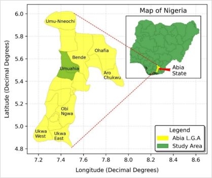
Figure 1. Map of Study Area.

2.2. Data Collection

The research employed a long-term rainfall dataset covering approximately three decades. A 31-year record from 1992 to 2022 was sourced from the Nigerian Meteorological Agency (NIMET) specifically for Umuahia. This dataset consisted of 24-hour daily rainfall measurements of the entire study, taken when it rained in Umuahia. Statistical methods were utilised to obtain each year's annual 24-hour maximum rainfall. To derive shorter rainfall duration records, the 24-hour data were downscaled using the Indian Meteorological Department (IMD) model, as outlined in Equation (1)

[15]

. The shorter duration records included 5, 10, 20, 30, 60, 120, 360, and 720 minutes.

R_{t}

R_{24} {(\frac{t}{24})}^{\frac{1}{3}}

(1)

Where

R_{t}

= Downscaled rainfall precipitation,

R_{24}

= daily rainfall precipitation (mm), t = time.

2.3. Development of Stationary and Non-Stationary IDF Rainfall Models

The magnitude of the extreme rainfall was computed using stationary and non-stationary approaches. Stationary approaches assume that the statistical parameters of the rainfall data remain constant over time, while non-stationary approaches assume that the statistical parameters vary over time. The magnitude of the extreme rainfall under stationarity was computed using Frequency Analysis

[20]

. Equation (2) was utilised to compute the magnitude of the extreme rainfall.

X_T=

\bar{x}

+ K_TS (2)

Where X_T= magnitude of the rainfall under a given time and return period,

\bar{x}

= mean of the rainfall at a particular time, S = standard deviation at a particular time, K_T= Frequency factor.

The frequency factor varies depending on the probability distribution. Table 1 gives the equations of frequency factors for three major probability distributions used for computing the magnitude of hydrologic events. Nwaogazie et al. detailed how frequency factors are used to obtain the magnitude of rainfall for five probability distributions

[12]

. The selection of the Frequency factor to utilise depends on how best the historical rainfall data fit the distribution. Kolmogorov Smirnov test was utilised to establish which distribution out of the four distributions considered, namely Gumbel EVT-1, Normal, Pearson Type -III, and Log Normal, fit the rainfall data best. Kolmogorov Smirnov test compares the cumulative distribution function of the rainfall data against the theoretical distribution function. The null hypothesis states that the dataset comes from a particular distribution been tested. If the computed D is greater than the critical value of the Kolmogorov-Smirnov statistic, then one rejects the null and states that the rainfall dataset does not come from that distribution. The best distribution with the less D value confirms that the rainfall dataset best fits that distribution, and the corresponding frequency factor would be utilised in obtaining the magnitude of the extreme rainfall (Equation (3)).

D =max|F_O(x) –F_t(x)| (3)

Table 1. Frequency factor for three probability distribution.

Distribution

Frequency Factors (K_T)

Gumbel EVT-1

K_T= $\frac{- \sqrt{6}}{π} [0.5772 + 1 n [In (T / T - 1)]]$ where T= return period

Normal

$K_{T} = z = w$ - $[\frac{2.525517 + 0.802853 w + 0.010328 w^{2}}{1 + 1.432788 w + 0.189269 w^{2} + 0.001308 w^{3}}]$

w = $\sqrt{1 n (+ \frac{1}{p 2})}$ for (0 < p ≤ 0.5) where p = 1/T

if p > 0.5, p is replaced with 1 – p

W = $\sqrt{In (\frac{1}{{(1 - p)}^{2}})}$

Pearson

K_T= Z + (Z²- 1) K + 1/3 (Z³-6) K^{2 –}(Z²-1) K³+ZK⁴+ 1/3 K⁵K= $\frac{c_{s}}{6}$ when C_{s ≠}0 where C_s= coefficient of skewness

Source:

[20]

The confirmation of non-stationarity in rainfall data is done using Mann Kendall which establish that there is a significant trend in the data

[17]

. Ekwueme et al. analysed the trend in rainfall data from 1992 to 2022 for Umuahia and confirmed the existence of an increasing trend in the rainfall for Umuahia

[7]

. The non-stationary IDF rainfall models were developed using the General Extreme Value (GEV) distribution

[18]

. This distribution was specifically adapted to model various behavioural extremes through three parameters namely: location, scale, and shape

[5]

. Equation (4) illustrates the GEV's standard cumulative distribution function (CDF) as provided by

[6]

F (x) = \exp [- {(1 + ξ (t) \frac{x - μ (t)}{σ (t)})}^{- \frac{- 1}{ξ (t)}}] for ξ \neq 0

(4)

Where F(x) = Cumulative distribution function,

μ

= mean (location),

σ

= standard deviation (scale) and,

ξ

= shape parameter are three behavioural parameter extremes.

The maximum likelihood estimator served as the statistical method for estimating distribution parameters due to its ability to adapt to non-stationary evaluations. Non-stationarity arises when one or more GEV statistical parameters are expressed as time functions

[6, 9]

. Three linear expressions of non-stationarity were employed to develop the IDF models, as detailed in Table 2. The best non-stationary model was chosen based on AIC and BIC goodness of fit criteria. The model with the lowest AIC and BIC best fit the rainfall's non-stationarity was deemed to adequately model the non-stationarity pattern in the rainfall data. Library (extRemes) in R-studio was used to derive the non-stationary model parameters and to calculate rainfall intensity.

Table 2. Types of Selected GEV Linear Parameter Models.

Model Type	Parameter Combination	Remark
(i) GEV_t – 0	$μ (t) = μ$ $σ (t) = σ$ $ξ (t) = ξ$	Stationary parameter model
(ii) GEV_t – I	$μ (t) = μ_{0} + μ_{1} t$ $σ (t) = σ$ $ξ (t) = ξ$ $μ (t) = μ$	Non-stationary parameter model
(iii) GEV_t – II	$σ (t) = σ_{0} + σ_{1} t$ $ξ (t) = ξ$ ${μ (t) = μ}_{0} + μ_{1} t$	Non-stationary parameter model
(iv) GEV_t – III	$μ (t) = μ_{0} + μ_{1} t$ $σ (t) = σ_{0} + σ_{1} t$ $ξ (t) = ξ$	Non-stationary parameter model

Source:

[19]

2.4. Comparative Analysis of Rainfall Intensity

Rainfall intensities were computed for various durations (5-1440 minutes) and return periods (2, 5, 10, 25, 50, and 100 years) to quantify differences between stationary and non-stationary approaches using both modelling approaches. Percentage differences were calculated using Equation (5):

Percentage diff (%) =

\frac{(NS - S)}{S} \times 100

(5)

Where NS = rainfall intensity from non-stationary model, S = rainfall intensity from stationary model.

3. Results

3.1. Stationary IDF Model Development

Visual inspection of the cumulative distribution function presented in Figure 2 revealed that the four theoretical cumulative distribution functions fit relatively well with the empirical cumulative distribution function. However, Gumbel EVT-1 (yellow line) was revealed to be the best fit as the maximum difference between the empirical and Gumbel EVT-1 CDF was relatively smaller than other theoretical CDFs. This was confirmed by the Kolmogorov-Smirnov test, as presented in Table 3. The result from Table 3 revealed that the maximum difference for the empirical CDF and Gumbel EVT-1 theoretical CDF was 0.09537 which was less than the critical value of 0.2443 at 5% significance level. The evidence provided by the K-S test informed the decision to develop the rainfall IDF model using Gumbel EVT-1 distribution. This finding aligns with hydrological theory, as the Gumbel distribution is widely recognised for its effectiveness in modelling extreme events such as annual maximum rainfall. Gumbel's superior performance compared to other distributions is likely due to its ability to capture the right-skewed nature of rainfall extremes in Umuahia's tropical climate.

Based on the selected Gumbel distribution, stationary IDF curves were developed for various durations and return periods. The K_T factor was computed for five return periods, and the rainfall intensities were computed for various durations and return periods, as presented in Table 4. Figure 3a presents the stationary IDF curves for shorter durations (5-60 minutes), which can be utilised to design urban culverts and drainage. Figure 3b shows IDF curves for longer durations (120-1440 minutes), which can be utilised for the design of bridges. The rainfall IDF curves exhibit the characteristic hyperbolic relationship between rainfall intensity and duration, with intensity decreasing as duration increases. Higher curves correspond to longer return periods, reflecting the increased rainfall intensity expected for less frequent events.

Download: Download full-size image

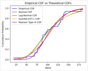
Figure 2. Empirical and theoretical Cumulative Distribution function.

Table 3. Kolmogorov-Smirnov Test Results for Distribution Fitting for Umuahia.

Time (mins)	Gumbel EVT-1	Normal	Log-Normal	Pearson Type III	Best Distribution Fit
5	0.09531	0.13975	0.11675	0.12762	Gumbel
10	0.09537	0.13983	0.11701	0.12997	Gumbel
20	0.09513	0.13998	0.11642	0.13051	Gumbel
30	0.09524	0.14012	0.11671	0.13121	Gumbel
60	0.09515	0.14010	0.11657	0.13045	Gumbel
120	0.09531	0.14002	0.11649	0.13043	Gumbel
360	0.09525	0.14001	0.11661	0.13100	Gumbel
720	0.09525	0.13994	0.11668	0.13116	Gumbel
1440	0.09525	0.13997	0.11661	0.13154	Gumbel

Critical value = 0.24426,

\propto

= 0.05. Bold values indicate that it was significant, while values highlighted with red indicate that the data best fit that distribution.

Table 4. Computed rainfall intensity using Gumbel Distribution.

Duration (mins)	Return Period (Years)
Duration (mins)	2	5	10	25	50	100
5	177.50	234.82	272.78	320.74	356.31	391.63
10	111.82	147.93	171.84	202.06	224.47	246.72
20	70.44	93.19	108.25	127.28	141.39	155.41
30	53.76	71.12	82.61	97.13	107.91	118.60
60	33.86	44.80	52.04	61.19	67.98	74.71
120	21.33	28.22	32.78	38.55	42.82	47.07
360	10.26	13.57	15.76	18.53	20.59	22.63
720	6.46	8.55	9.93	11.67	12.97	14.25
1440	4.07	5.38	6.25	7.35	8.17	8.98

Download: Download full-size image

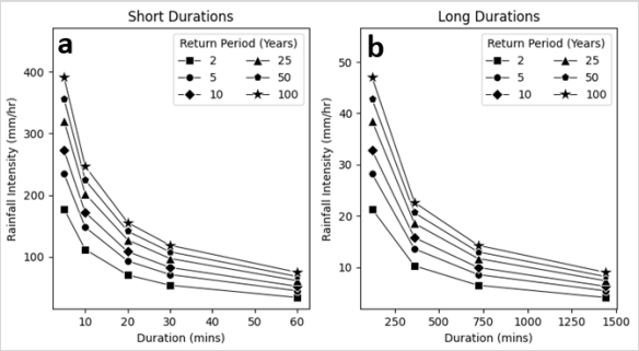
Figure 3. Stationary IDF Curves for Shorter Durations (5-60 minutes) and for Longer Durations (120-1440 minutes).

3.2. Non-Stationary IDF Model Development

Non-stationary model assumes that the rainfall parameters change over time. Ekwueme et al. confirmed that the rainfall for Umuahia from 1992 to 2022 had an increasing trend, with a change point year established around 2002

[7]

. This evidence of an increasing trend in rainfall in Umuahia provided sufficient evidence for developing rainfall models utilising a non-stationary approach. Table 5 presents the rainfall models developed using the non-stationary IDF approach. An analysis of the GEV parameters uncovers notable patterns across various time durations, ranging from 5 to 1440 minutes. For the 5-minute duration, the GEVt-I model provided the best fit, evidenced by the lowest AIC value of 196.264 and a BIC of 202.00. This trend of GEVt-I outperforming other models is consistent across all durations, as it repeatedly achieves the lowest AIC values. The models displayed similar behaviours for intermediate durations (10-60 minutes). In the analysis for 10 minutes, the GEVt-I model also performed optimally with an AIC of 212.487. This pattern continued for the 20-minute (AIC = 227.338) and the 30-minute (AIC = 236.338), where the location parameters adjusted gradually while preserving the model's superior fit. For longer durations (120-1440 minutes), GEVt-I remained the top performer, with the 720-minute duration analysis yielding an AIC of 302.018, and the 1440-minute duration presenting an AIC of 316.344, both reflecting the lowest values in their respective duration categories. The performance of the GEVt -I model suggests that the mean of the rainfall steadily increases over time, but there was little variation in the rainfall over time. The computed rainfall intensity utilising the non-stationary model is presented in Table 6. The non-stationary IDF curves is shown in Figure 4 which revealed similar trend with the stationary model. Increase in the duration would result in the reduction of the rainfall intensity for a particular return period. Also, increase in the return period would result to a more intense rainfall intensity for a particular duration.

Table 5. Evaluation of the performance of GEV parameters used for non-stationary and stationary models for Umuahia.

Time (mins)	Models	Location Parameter	Scale	Shape Parameter	BIC	AIC
5	GEV_t– I	-181.219 + 0.097t	4.766	-0.204	202.00	196.264
	GEV_t– II	13.694	4.907 – 0.0001t	-0.231	205.06	199.319
	GEV_t- III	-241.848 + 0.127t	14.439– 0.005t	-0.204	204.94	197.766
10	GEV_t– I	-63.339 + 0.040t	6.306	-0.222	218.222	212.487
	GEV_t– II	17.253	6.182 - 0.0002t	-0.231	219.386	213.650
	GEV_t- III	-188.624 + 0.103t	13.781– 0.004t	-0.210	220.125	212.955
20	GEV_t– I	-31.406 + 0.027t	8.0489	-0.225	233.074	227.338
	GEV_t– II	21.737	7.787 + 0.0002t	-0.231	233.700	227.964
	GEV_t- III	-3.476+1.841t	2.028– 0.0006t	-0.218	233.623	226.453
30	GEV_t– I	24.015 + 0.0004t	9.424	-0.230	242.075	236.338
	GEV_t– II	24.884	8.915 + 0.0002t	-0.231	242.082	236.347
	GEV_t- III	-63.906 + 0.044t	12.204– 0.002t	-0.236	244.682	237.512
60	GEV_t– I	23.921 + 0.0037t	11.865	-0.233	256.343	250.607
	GEV_t– II	31.523	11.24 + 0.0003t	-0.231	256.404	250.668
	GEV_t- III	-487.80 + 0.259t	31.580– 0.010t	-0.211	256.38	249.214
120	GEV_t– I	36.189 + 0.0017t	14.909	-0.232	270.707	264.971
	GEV_t– II	39.503	14.15 + 0.0004t	-0.231	270.729	264.993
	GEV_t- III	-53.978 + 0.047t	17.478 – 0.002t	-0.227	273.55	266.385
360	GEV_t– I	56.024 + 0.0005t	21.489	-0.231	293.428	287.692
	GEV_t– II	56.978	20.41 + 0.0005t	-0.231	293.432	287.696
	GEV_t- III	-30.889 + 0.044t	23.496– 0.001t	-0.239	296.475	289.305
720	GEV_t– I	70.603 + 0.0006t	27.078	-0.232	307.754	302.018
	GEV_t– II	71.787	25.71 + 0.0007t	-0.232	307.759	302.023
	GEV_t- III	20.065 + 0.0259t	27.47– 0.0003t	-0.231	311.005	303.835
1440	GEV_t– I	88.962 + 0.0008t	34.120	-0.232	322.080	316.344
	GEV_t– II	90.478	32.39 + 0.0009t	-0.232	322.085	316.349
	GEV_t- III	88.902 + 0.008t	32.40 + 0.0009t	-0.232	325.514	318.344

Table 6. Computed rainfall intensity for the non-stationary model for Umuahia.

Duration (mins)	Return Period (Years)
Duration (mins)	2	5	10	25	50	100
5	203.54	257.24	286.54	317.69	337.20	353.98
10	120.71	155.66	174.40	194.01	206.11	216.39
20	81.82	103.16	114.66	126.74	134.23	140.60
30	56.41	73.69	82.89	92.45	98.31	103.26
60	39.29	49.56	55.13	61.01	64.68	67.82
120	22.40	29.22	32.85	36.61	38.92	40.86
360	10.76	14.04	15.79	17.60	18.71	19.64
720	6.78	8.85	9.94	11.09	11.78	12.37
1440	4.27	5.57	6.26	6.98	7.42	7.79

Download: Download full-size image

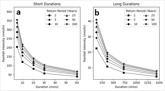
Figure 4. Non-Stationary IDF Curves for Shorter Durations (5-60 minutes) and for Longer Durations (120-1440 minutes).

3.3. General IDF Models

Table 7 summarizes the general IDF models developed for both stationary and non-stationary approaches. These models are based on the modified Sherman's equation format, which mathematically represents the relationship among rainfall intensity, duration, and return period. Both models exhibit impressive performance metrics. The stationary model attained a coefficient of determination (R²) of 0.998, suggesting it accounts for 99.8% of the variance in rainfall intensity. Its mean squared error (MSE) was 19.93, indicating strong prediction accuracy. Meanwhile, the non-stationary model produced a marginally lower R² of 0.992 and an MSE of 38.09, which is still notably high. These general models provide engineers and hydrologists with readily applicable equations for determining rainfall intensities for any duration and return period without referencing or interpolating from IDF curve graphs.

Table 7. GEV fitted General for Stationary and Non-stationary IDF (GNS-IDF) models for Umuahia.

S/N	Stations	IDF Models	R²	MSE
1	Stationary	I = $\frac{502.251 T_{r}^{0.184}}{T_{d}^{0.6667}}$	0.998	19.93
2	Non-Stationary	I = $\frac{315.26 T_{r}^{0.315}}{T_{d}^{0.685}}$	0.992	38.09

3.4. Comparative Analysis of Rainfall Intensity Between Stationary and Non-Stationary Models

The rainfall intensity obtained from stationary and non-stationary models are presented in Figure 5. The result from Figure 5 revealed that the non-stationary model produces a higher rainfall intensity for the shorter return period (2 to 10 years). But for longer return periods, the stationary model produced higher rainfall intensity. The result of the percentage difference in the rainfall intensity for all durations and return periods is presented in Table 8. The percentage difference in the 2-year return period ranged from 4.93 - 16.16%, with the largest differences observed for 20 and 60 minutes. For the 5-year return period, differences ranged from 3.49 - 10.71%, and for the 10-year return period, from 0.16 - 5.93%.

Download: Download full-size image

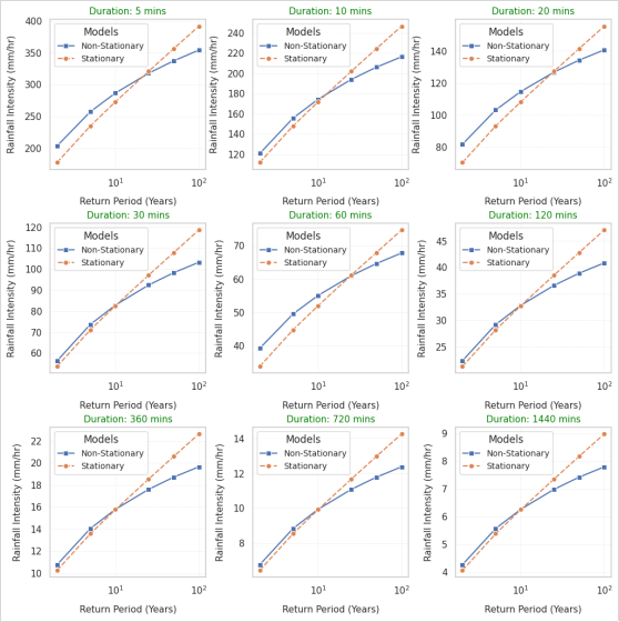
Figure 5. Rainfall Intensity for Stationary and Non-Stationary models.

Table 8. Percentage Difference in Rainfall Intensity Between Non-Stationary and Stationary IDF Models for Umuahia.

Duration (mins)	Significant Trend	Significant Change Point	Return Period (Years)
Duration (mins)	Significant Trend	Significant Change Point	2	5	10	25	50	100
5	Yes	Yes (2002-2003)	14.670	9.550	5.050	-0.950	-5.360	-9.610
10	Yes	Yes (2002-2003)	7.960	5.220	1.490	-3.980	-8.180	-12.290
20	Yes	Yes (2002-2003)	16.160	10.710	5.920	-0.420	-5.070	-9.530
30	Yes	Yes (2002-2003)	4.930	3.620	0.330	-4.820	-8.890	-12.930
60	Yes	Yes (2002-2003)	16.010	10.620	5.930	-0.290	-4.850	-9.230
120	Yes	Yes (2002-2003)	5.000	3.550	0.200	-5.020	-9.120	-13.180
360	Yes	Yes (2002-2003)	4.930	3.490	0.160	-5.040	-9.130	-13.180
720	Yes	Yes (2002-2003)	4.930	3.500	0.160	-5.040	-9.140	-13.200
1440	Yes	Yes (2002-2003)	4.940	3.500	0.160	-5.050	-9.150	-13.210
Average	-	-	8.840	5.970	2.150	-3.400	-7.650	-11.820

The pattern reversed for longer return periods (25-100 years), with stationary models generally predicting higher intensities than non-stationary models. At the 25-year return period, differences ranged from -0.29 to -5.05%. Differences were more pronounced for the 50-year return period, ranging from -4.85 to -9.15%. At the 100-year return period, the percentage differences ranged from -9.23 to -13.21%, indicating that stationary models may overestimate extreme rainfall events for very long return periods.

The average percentage differences across all durations were 8.84% for the 2-year return period, 5.97% for the 5-year return period, 2.15% for the 10-year return period, -3.40% for the 25-year return period, -7.65% for the 50-year return period, and -11.82% for the 100-year return period. This pattern of decreasing and eventually negative differences with increasing return period is consistent across all durations, suggesting a systematic relationship between the return period and the relative performance of stationary versus non-stationary models in Umuahia. The rainfall duration seems to exert a less consistent influence on the discrepancies between models compared to the return period. However, the 20 and 60-minute durations consistently demonstrate the most significant positive differences at shorter return periods, indicating this intermediate length (time interval) might be especially responsive to the non-stationary effects addressed by the time-dependent model.

4. Discussion

The comparative analysis of stationary and non-stationary IDF models reveals significant patterns that have important implications for infrastructure design and flood risk management in South-Eastern Nigeria. The finding from the result revealed that the non-stationary model predicted higher rainfall intensities for shorter return periods (2-10 years), indicating the need for developing IDF model adopting a non-stationary approach. Rainfall intensity at shorter durations and return periods is particularly useful for urban drainage design. A significant difference is highlighted at the 20-minute duration for the 2 and 5-year return periods, with non-stationary models predicting rainfall intensities of 16.16 and 10.71% greater than those from stationary models. This specific duration and return period range is critically important, representing the standard design criteria for residential and urban drainage systems. The findings suggest that Umuahia's existing drainage system, developed with a stationary rainfall model, might be significantly inadequate for current rainfall patterns, which could account for the rise in localised flooding observed in recent years.

The pattern of higher non-stationary intensities for frequent events and lower non-stationary intensities for rare events aligns with climate change projections that suggest an intensification of common rainfall events. Ganguli and Coulibaly observed that the rainfall intensity obtained from the non-stationary model was higher than the stationary one for most locations in Canada, especially for shorter return periods

[8]

. The percentage difference for shorter durations ranged from 1 to 14%, which was lower than the percentage difference obtained in the current study. Ganguli and Coulibaly argued that the lack of significant difference between the rainfall intensity obtained from the non-stationary and stationary models should not prompt the development of IDF relationships using a non-stationary approach

[8]

. However, this view can create problems, judging from the reasonable size percentage differences of 16% observed between stationary and non-stationary rainfall intensity for a design storm intensity of 20 minutes’ duration for a 2-year return period in the current study. Cheng & AghaKouchak also observed that the non-stationary model produced higher rainfall intensity, particularly for shorter return periods

[4]

. They argued that the climate change projection or trend should dictate the use of non-stationary approach rather than the statistically significant difference observed between the rainfall intensity between the two approaches. Xu et al. reported that nonstationary models produced higher design storm intensity, DSI than stationary ones and attributed the higher DSI in nonstationary models to rapid urban development in the location

[21]

From an engineering standpoint, these findings directly impact infrastructure design standards. Existing drainage systems, which are built for 2 to 10-year return periods using stationary assumptions, may be undersized by about 5 -16%. This shortcoming raises the likelihood of flooding during regular rainfall events. Thus, it is essential for engineering design standards to integrate non-stationary models, especially for infrastructure with shorter design return periods.

The findings indicate that climate change adaptation strategies in Umuahia must focus on enhancing urban drainage systems built for shorter return periods, as they demonstrate the most significant underestimation when applying stationary assumptions. Conversely, the existing stationary approaches yield more conservative estimates for major infrastructures meant to endure longer return periods (25-100 years). Identifying specific durations and return periods where differences are most pronounced provides valuable guidance for prioritising adaptation efforts in South-Eastern Nigeria.

5. Conclusion

The research investigated the difference between stationary and non-stationary rainfall IDF models in Umuahia, the capital of Abia state, Nigeria. The results indicate that the non-stationary model forecasted greater rainfall intensities for shorter return periods (2-10 years), highlighting the need for an IDF model employing a non-stationary approach. The rainfall intensity predictions for shorter durations and return periods are especially valuable for urban drainage design. The trend of higher non-stationary intensities for more frequent events (shorter return periods) gives an indication of a changing climate for more frequent hydrologic events. From an engineering perspective, these insights directly affect infrastructure design standards. Current drainage systems, which are designed for 2 to 10-year return periods based on stationary assumptions, could be insufficient by approximately 5-16%. This gap increases the risk of flooding during typical rainfall events. Therefore, it is important for engineering design standards to incorporate non-stationary models, particularly for infrastructures designed with shorter return periods.

Abbreviations

CDF	Cumulative Distribution Function
DSI	Design Storm Intensity
EVt	Extreme Value Type
GEV	General Extreme Value
GNS-IDF	General Non-stationary Intensity Duration Frequency
IDF	Intensity Duration Frequency
IMD	Indian Meteorological Department model
K-S	Kolmogorov-Smirnov
NIMET	Nigerian Meteorological Agency
NS-IDF	Non-stationary Intensity Duration Frequency

Author Contributions

Chimeme Martin Ekwueme: Conceptualization, Investigation, Methodology, Validation, Writing – original draft

Ify LawrenceNwaogazie: Conceptualization, Supervision, Validation, Writing – review & editing

Chiedozie Francis Ikebude: Conceptualization, Supervision, Validation, Writing – review & editing

Godwin Otunyo Amuchi: Funding acquisition, Writing – review & editing

Jonathan Onyekachi Irokwe: Funding acquisition, Writing – review & editing

Conflicts of Interest

The authors declare no conflicts of interest.

References

[1]	Abiodun, B. J., Adegoke, J., Abatan, A. A., Ibe, C. A., Egbebiyi, T. S., Engelbrecht, F. & Pinto, I. (2017). Potential impacts of climate change on extreme precipitation over four African coastal cities. Climate change (2017) 143: 399-413. https://doi.org/10.1007/s10584-017-2001-5
[2]	AghaKouchak, A., Ragno, E., Love, C. & Moftakhari, H. (2018). Projected Changes in California's precipitation intensity-duration-frequency curves. California's fourth climate change assessment, California energy commission. Pub. No.: CCCA4-CEC- 2018-005.
[3]	Akinsanola, A. A. & Ogunjobi, K. O. (2015). Recent homogeneity analysis and long-term spatio-temporal rainfall trends in Nigeria. Theoretical and Applied Climatology, 128, 275-289.
[4]	Cheng, L. & AghaKouchak, A. (2014). Non-stationarity precipitation intensity-duration-frequency curves for infrastructure design in a changing climate. Science Reports, 4(7093), 1-6.
[5]	Cheng, L., AghaKouchak, A., Gilleland, E. & Katz, R. W. (2014). Non-stationary extreme value analysis in a changing climate. Climate Change, 127(2), 353-369.
[6]	Coles, S., Bawa, J., Trenner, L. & Dorazio, P. (2001). An introduction to statistical modeling of extreme values. London: Springer.
[7]	Ekwueme, C. M., Nwaogazie, I. L., Ikebude, C. F., Amuchi, G. O., Irokwe, J. O., et al. (2025). Modeling Rainfall Intensity-Duration-Frequency (IDF) and Establishing Climate Change Existence in Umuahia - Nigeria Using Non-Stationary Approach. Hydrology, 13(1), 83-89. https://doi.org/10.11648/j.hyd.20251301.19
[8]	Ganguli, P. & Coulibaly, P. (2017). Does non-stationarity in rainfall require non-stationary intensity-duration-frequency curves? Hydrology and Earth System Sciences, 21, 6461-6483.
[9]	Katz, R. W. (2013). Statistical methods for nonstationary extremes. In: Extremes in a changing climate (pp. 15-37). Dordrecht: Springer.
[10]	Masi, M., Kanakoudis, V., & Salcedo, A. G. (2023). Statistical, Analytical and Numerical Approaches for the Design of Urban Drainage Systems under Climate Change Conditions. Climate, 11(7), 141. https://doi.org/10.3390/cli11070141
[11]	Milly, P. C. D., Betancourt, J., Falkenmark, M., Hirsch, R. M., Kundzewicz, Z. W., Lettenmaier, D. P. & Stouffer, R. J. (2008). Stationarity is dead: Whither water management? Science, 319(5863), 573-574. https://doi.org/10.1126/science.1151915
[12]	Nwaogazie, I. L., Sam, M. G., Enciso, R. Z., & Gonsalves, E. (2019). Probability and non-probability rainfall intensity-duration-frequency modeling for Port-Harcourt metropolis, Nigeria. International Journal of Hydrology, 3(1), 66-75.
[13]	Odjugo, P. A. O. (2013). Analysis of climate change awareness in Nigeria. Science Research Essays, 8(26), 1203-1211.
[14]	Ouarda, T. B. M. J., Yousef, L. A. & Charron, C. (2019). Non-stationary intensity-duration-frequency curves integrating information concerning teleconnections and climate change. International Journal of Climatology, 39, 2306-2323. https://doi.org/10.1002/joc.5953
[15]	Sam M. G, Nwaogazie I. L. and Ikebude, C. (2021): Improving Indian meteorological department method for 24- hourly rainfall downscaling to shorter durations for IDF modelling. International Journal of Hydrology; 5(2): 72-82. https://doi.org/10.15406/ijh.2021.05.00268
[16]	Sam, M. G., Nwaogazie, I. L., Ikebude, C., Inyang, U. J. and Irokwe, J. O. (2023a). Modeling Rainfall Intensity-Duration-Frequency (IDF) and Establishing Climate Change Existence in Uyo-Nigeria Using Non-Stationary Approach. Journal of water Resource and protection, Vol. 15, pp 194-214.
[17]	Sam, M. G., Nwaogazie, I. L., & Ikebude, C. (2023b). Establishing Climatic Change on Rainfall Trend, Variation and Change Point Pattern in Benin City, Nigeria. International Journal of Environment and Climate Change, 13(5), 202-212.
[18]	Sam, M. G., Nwaogazie, I. L., & Ikebude, C. (2023c). General extreme value fitted rainfall non-stationary intensity-duration-frequency (NS-IDF) modelling for establishing climate change in Benin City. Hydrology, 11(4), 85-93.
[19]	Silva, D. F. & Simonovic, S. P. (2020). Development of non-stationary rainfall intensity duration frequency curves for future climate conditions. Water resources research report No: 106. Department of civil and environmental engineering, western University, Canada.
[20]	Te Chow, V., Maidment, D. R., & Mays, L. W. (1988). Solutions Manual to Accompany Applied Hydrology. McGraw-Hill.
[21]	Xu, P., Wang, D., Wang, Y., Wu, J., Heng, Y., Singh, V. P.,... & Fang, H. (2024). Quantifying the urbanization and climate change-induced impact on changing patterns of rainfall Intensity-Duration-Frequency via nonstationary models. Urban Climate, 55, 101990. RetryClaude does not have internet access. Links provided may not be accurate or up to date.

Cite This Article

Plain Text BibTeX RIS

APA Style

Ekwueme, C. M., Nwaogazie, I. L., Ikebude, C. F., Amuchi, G. O., Irokwe, J. O. (2025). Comparative Analyses of Stationary and Non-Stationary IDF Rainfall Models for Umuahia. Hydrology, 13(2), 102-113. https://doi.org/10.11648/j.hyd.20251302.12

Copy | Download

ACS Style

Ekwueme, C. M.; Nwaogazie, I. L.; Ikebude, C. F.; Amuchi, G. O.; Irokwe, J. O. Comparative Analyses of Stationary and Non-Stationary IDF Rainfall Models for Umuahia. Hydrology. 2025, 13(2), 102-113. doi: 10.11648/j.hyd.20251302.12

Copy | Download

AMA Style

Ekwueme CM, Nwaogazie IL, Ikebude CF, Amuchi GO, Irokwe JO. Comparative Analyses of Stationary and Non-Stationary IDF Rainfall Models for Umuahia. Hydrology. 2025;13(2):102-113. doi: 10.11648/j.hyd.20251302.12

Copy | Download

@article{10.11648/j.hyd.20251302.12,
  author = {Chimeme Martin Ekwueme and Ify Lawrence Nwaogazie and Chiedozie Francis Ikebude and Godwin Otunyo Amuchi and Jonathan Onyekachi Irokwe},
  title = {Comparative Analyses of Stationary and Non-Stationary IDF Rainfall Models for Umuahia
},
  journal = {Hydrology},
  volume = {13},
  number = {2},
  pages = {102-113},
  doi = {10.11648/j.hyd.20251302.12},
  url = {https://doi.org/10.11648/j.hyd.20251302.12},
  eprint = {https://article.sciencepublishinggroup.com/pdf/10.11648.j.hyd.20251302.12},
  abstract = {This study aimed to develop IDF models and compare rainfall intensity obtained from the stationary and non-stationary IDF models for Umuahia in South-Eastern Nigeria. The research used a long-term rainfall dataset spanning three decades (1992-2022) sourced from the Nigerian Meteorological Agency. The daily rainfall data recorded over 24 hours was downscaled to shorter periods using the Indian Meteorological Department model (IMD). For determining the best distribution fitting for the rainfall data, the Kolmogorov-Smirnov (K-S) test was utilised. The result from the K-S test revealed that Gumbel EVT-1 was the best-fitting distribution for creating the stationary IDF models. The GEVt-I model, which includes a time-dependent location parameter, proved the most effective for non-stationary models. The comparative analysis showed that non-stationary models forecasted greater rainfall intensities for shorter return periods (2-10 years), with variations between 4.93 and 16.16% for the 2-year return period. In contrast, for longer return periods (25-100 years), stationary models yielded higher intensity predictions, with differences ranging from -0.29 -13.21%. These results have important implications for infrastructure design and flood risk management in Umuahia, indicating that existing drainage systems based on stationary assumptions may be undersized by 5-16%, which could elevate the risk of flooding during typical rainfall events.
},
 year = {2025}
}

Copy | Download

TY  - JOUR
T1  - Comparative Analyses of Stationary and Non-Stationary IDF Rainfall Models for Umuahia

AU  - Chimeme Martin Ekwueme
AU  - Ify Lawrence Nwaogazie
AU  - Chiedozie Francis Ikebude
AU  - Godwin Otunyo Amuchi
AU  - Jonathan Onyekachi Irokwe
Y1  - 2025/04/29
PY  - 2025
N1  - https://doi.org/10.11648/j.hyd.20251302.12
DO  - 10.11648/j.hyd.20251302.12
T2  - Hydrology
JF  - Hydrology
JO  - Hydrology
SP  - 102
EP  - 113
PB  - Science Publishing Group
SN  - 2330-7617
UR  - https://doi.org/10.11648/j.hyd.20251302.12
AB  - This study aimed to develop IDF models and compare rainfall intensity obtained from the stationary and non-stationary IDF models for Umuahia in South-Eastern Nigeria. The research used a long-term rainfall dataset spanning three decades (1992-2022) sourced from the Nigerian Meteorological Agency. The daily rainfall data recorded over 24 hours was downscaled to shorter periods using the Indian Meteorological Department model (IMD). For determining the best distribution fitting for the rainfall data, the Kolmogorov-Smirnov (K-S) test was utilised. The result from the K-S test revealed that Gumbel EVT-1 was the best-fitting distribution for creating the stationary IDF models. The GEVt-I model, which includes a time-dependent location parameter, proved the most effective for non-stationary models. The comparative analysis showed that non-stationary models forecasted greater rainfall intensities for shorter return periods (2-10 years), with variations between 4.93 and 16.16% for the 2-year return period. In contrast, for longer return periods (25-100 years), stationary models yielded higher intensity predictions, with differences ranging from -0.29 -13.21%. These results have important implications for infrastructure design and flood risk management in Umuahia, indicating that existing drainage systems based on stationary assumptions may be undersized by 5-16%, which could elevate the risk of flooding during typical rainfall events.

VL  - 13
IS  - 2
ER  -

Copy | Download

Author Information

Chimeme Martin Ekwueme

Department of Civil and Environmental Engineering, University of Calabar, Calabar, Nigeria

http://orcid.org/0009-0008-0168-0251
Ify Lawrence Nwaogazie

Department of Civil and Environmental Engineering, University of Port Harcourt, Port Harcourt, Nigeria

Contact Email

http://orcid.org/0000-0001-9480-1658
Chiedozie Francis Ikebude

Department of Civil and Environmental Engineering, University of Port Harcourt, Port Harcourt, Nigeria

http://orcid.org/0009-0006-7579-0950
Godwin Otunyo Amuchi

Department of Civil and Environmental Engineering, University of Port Harcourt, Port Harcourt, Nigeria
Jonathan Onyekachi Irokwe

Department of Civil and Environmental Engineering, University of Port Harcourt, Port Harcourt, Nigeria

http://orcid.org/0009-0001-7718-4915

Download PDF

Submit an Article

Plain Text BibTeX RIS

APA Style

Ekwueme, C. M., Nwaogazie, I. L., Ikebude, C. F., Amuchi, G. O., Irokwe, J. O. (2025). Comparative Analyses of Stationary and Non-Stationary IDF Rainfall Models for Umuahia. Hydrology, 13(2), 102-113. https://doi.org/10.11648/j.hyd.20251302.12

Copy | Download

ACS Style

Ekwueme, C. M.; Nwaogazie, I. L.; Ikebude, C. F.; Amuchi, G. O.; Irokwe, J. O. Comparative Analyses of Stationary and Non-Stationary IDF Rainfall Models for Umuahia. Hydrology. 2025, 13(2), 102-113. doi: 10.11648/j.hyd.20251302.12

Copy | Download

AMA Style

Ekwueme CM, Nwaogazie IL, Ikebude CF, Amuchi GO, Irokwe JO. Comparative Analyses of Stationary and Non-Stationary IDF Rainfall Models for Umuahia. Hydrology. 2025;13(2):102-113. doi: 10.11648/j.hyd.20251302.12

Copy | Download

@article{10.11648/j.hyd.20251302.12,
  author = {Chimeme Martin Ekwueme and Ify Lawrence Nwaogazie and Chiedozie Francis Ikebude and Godwin Otunyo Amuchi and Jonathan Onyekachi Irokwe},
  title = {Comparative Analyses of Stationary and Non-Stationary IDF Rainfall Models for Umuahia
},
  journal = {Hydrology},
  volume = {13},
  number = {2},
  pages = {102-113},
  doi = {10.11648/j.hyd.20251302.12},
  url = {https://doi.org/10.11648/j.hyd.20251302.12},
  eprint = {https://article.sciencepublishinggroup.com/pdf/10.11648.j.hyd.20251302.12},
  abstract = {This study aimed to develop IDF models and compare rainfall intensity obtained from the stationary and non-stationary IDF models for Umuahia in South-Eastern Nigeria. The research used a long-term rainfall dataset spanning three decades (1992-2022) sourced from the Nigerian Meteorological Agency. The daily rainfall data recorded over 24 hours was downscaled to shorter periods using the Indian Meteorological Department model (IMD). For determining the best distribution fitting for the rainfall data, the Kolmogorov-Smirnov (K-S) test was utilised. The result from the K-S test revealed that Gumbel EVT-1 was the best-fitting distribution for creating the stationary IDF models. The GEVt-I model, which includes a time-dependent location parameter, proved the most effective for non-stationary models. The comparative analysis showed that non-stationary models forecasted greater rainfall intensities for shorter return periods (2-10 years), with variations between 4.93 and 16.16% for the 2-year return period. In contrast, for longer return periods (25-100 years), stationary models yielded higher intensity predictions, with differences ranging from -0.29 -13.21%. These results have important implications for infrastructure design and flood risk management in Umuahia, indicating that existing drainage systems based on stationary assumptions may be undersized by 5-16%, which could elevate the risk of flooding during typical rainfall events.
},
 year = {2025}
}

Copy | Download

TY  - JOUR
T1  - Comparative Analyses of Stationary and Non-Stationary IDF Rainfall Models for Umuahia

AU  - Chimeme Martin Ekwueme
AU  - Ify Lawrence Nwaogazie
AU  - Chiedozie Francis Ikebude
AU  - Godwin Otunyo Amuchi
AU  - Jonathan Onyekachi Irokwe
Y1  - 2025/04/29
PY  - 2025
N1  - https://doi.org/10.11648/j.hyd.20251302.12
DO  - 10.11648/j.hyd.20251302.12
T2  - Hydrology
JF  - Hydrology
JO  - Hydrology
SP  - 102
EP  - 113
PB  - Science Publishing Group
SN  - 2330-7617
UR  - https://doi.org/10.11648/j.hyd.20251302.12
AB  - This study aimed to develop IDF models and compare rainfall intensity obtained from the stationary and non-stationary IDF models for Umuahia in South-Eastern Nigeria. The research used a long-term rainfall dataset spanning three decades (1992-2022) sourced from the Nigerian Meteorological Agency. The daily rainfall data recorded over 24 hours was downscaled to shorter periods using the Indian Meteorological Department model (IMD). For determining the best distribution fitting for the rainfall data, the Kolmogorov-Smirnov (K-S) test was utilised. The result from the K-S test revealed that Gumbel EVT-1 was the best-fitting distribution for creating the stationary IDF models. The GEVt-I model, which includes a time-dependent location parameter, proved the most effective for non-stationary models. The comparative analysis showed that non-stationary models forecasted greater rainfall intensities for shorter return periods (2-10 years), with variations between 4.93 and 16.16% for the 2-year return period. In contrast, for longer return periods (25-100 years), stationary models yielded higher intensity predictions, with differences ranging from -0.29 -13.21%. These results have important implications for infrastructure design and flood risk management in Umuahia, indicating that existing drainage systems based on stationary assumptions may be undersized by 5-16%, which could elevate the risk of flooding during typical rainfall events.

VL  - 13
IS  - 2
ER  -

Copy | Download